
Aquatic and Terrestrial Pollution
APES Unit 8 Study Notes
Trace pollutants. Understand their impacts.
Review water pollution, waste, toxicology and environmental health with detailed notes, clear diagrams and worked calculations.
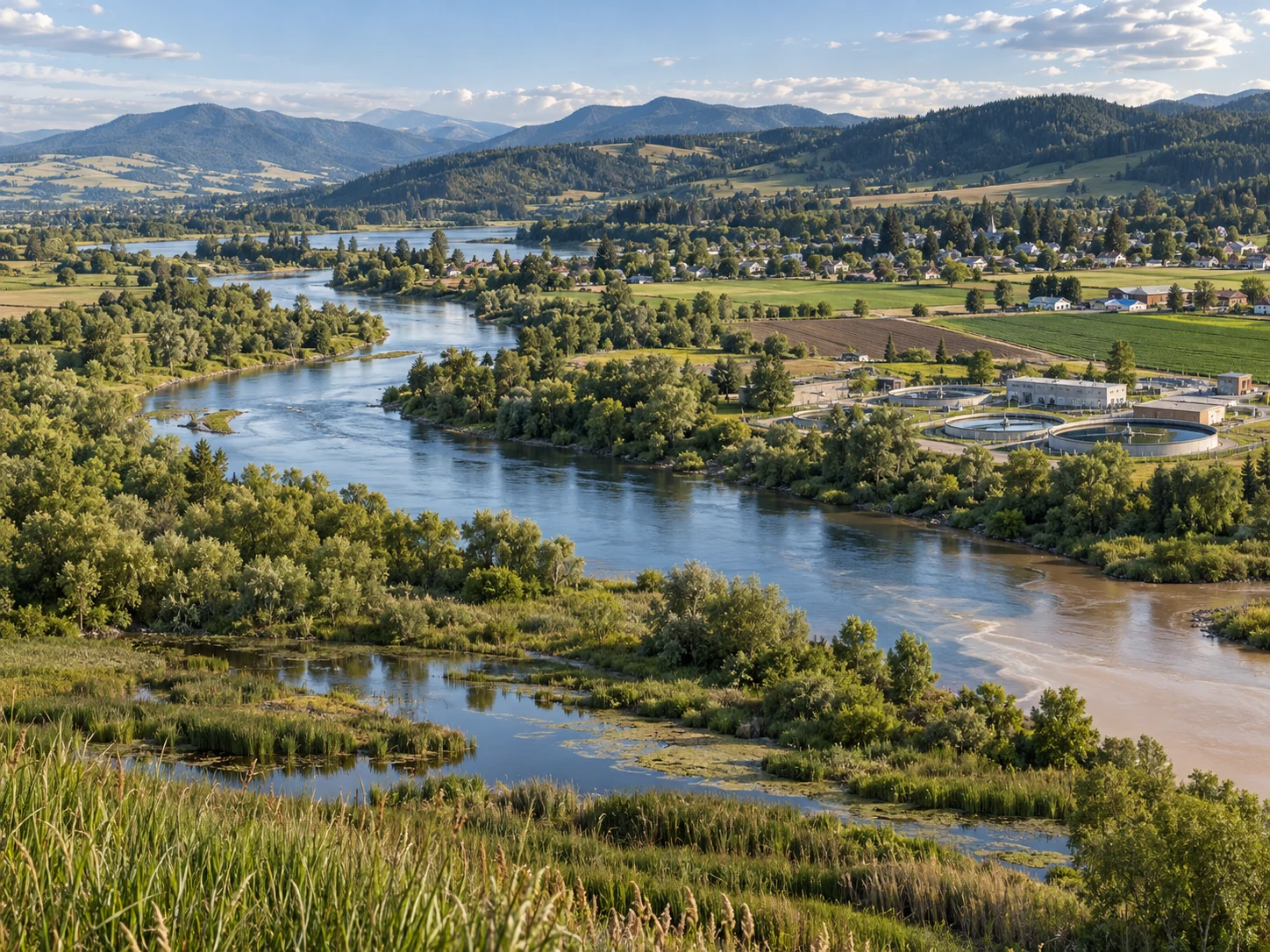
8.1 Sources of Pollution
Point vs. Nonpoint Pollution
Pollution sources are classified as point (specific location, traceable) or nonpoint (diffuse, widespread, difficult to trace). This distinction is critical for regulation and remediation strategies.
Point Source Pollution
- Definition: A point source is a discernible, confined conveyance such as a discharge pipe or channel. In the United States, the NPDES program regulates covered pollutant discharges to waters of the United States; air emissions use different regulatory programs.
- Examples: Wastewater-treatment outfalls, industrial pipes and regulated storm-sewer discharges. Leaking tanks and landfill leachate are contamination sources, but their legal classification depends on the release pathway and applicable law.
- Characteristics: A defined outlet supports flow measurement, sampling and source-specific controls. Monitoring can still be difficult, and a point discharge is not inherently cleaner than diffuse runoff.
- Pollutants: Heavy metals, organic chemicals, suspended solids, nutrients (N, P), pathogens, thermal discharge
- Advantages for Regulation: Traceable to source; technology-based controls applicable; Easy to hold responsible party liable
- Challenge: Multiple point sources add up; cumulative effect from many plants can be severe
Nonpoint Source Pollution
- Definition: Nonpoint pollution reaches water through diffuse pathways such as runoff, erosion, seepage or atmospheric deposition. Its contribution varies by watershed, pollutant and assessment method; there is no single global point–nonpoint percentage.
- Examples: Agricultural runoff (fertilizers, pesticides, eroded soil), urban stormwater (oil, sediment, metals from streets), atmospheric deposition, grazing animal waste, road salt
- Characteristics: Varies temporally (worse after rain); spatially distributed; multiple sources; difficult/expensive to monitor; hard to regulate individual contributors
- Pollutants: Nutrients (nitrogen, phosphorus from fertilizers), sediment (erosion), pesticides, pathogens, oil/grease, heavy metals
- Agriculture: Fertilizer, manure, soil and pesticide losses can be major watershed inputs. Source importance differs among rivers, lakes and wetlands; management should use local loads and impairment evidence.
- Stormwater: Runoff washes pollutants from impervious surfaces. A concentrated storm-sewer outlet may be a regulated point source even though pollutants originated across a broad area. First-flush effects vary among storms and pollutants.
- Challenge for Regulation: No clear responsible party; voluntary best management practices common; enforcement difficult; watershed-scale coordination needed
- Control Strategies: BMPs (best management practices): cover crops, buffer strips, sediment traps, urban green infrastructure; effectiveness variable
Major Pollutant Categories
Nutrient Pollution
- Sources: Fertilizer and manure losses, sewage, septic systems and atmospheric deposition supply nutrients in varying proportions. A watershed budget must define the nutrient, period and geographic boundary before assigning shares.
- Forms: Nitrogen (as nitrate, ammonium), Phosphorus (phosphate); both essential for growth but excessive in water
- Impact: Eutrophication (lake aging, excessive algae), dead zones (Gulf of Mexico, Baltic Sea), fisheries collapse
- Scale: Nutrient enrichment affects many fresh and coastal waters. Counts of hypoxic zones depend on survey coverage, oxygen threshold and year; distinguish a mapped area from the frequency and duration of oxygen depletion.
Sediment Pollution
- Sources: Exposed agricultural, construction, logging and mining soils, plus eroding streambanks, supply sediment. Rainfall, soil properties, slope and vegetation determine local erosion rates.
- Transport: Eroded soil can be stored on hillslopes or floodplains before reaching water. Soil-loss totals are not identical to sediment delivered to rivers; sediment loads need a catchment and period.
- Effects: Turbidity reduces light (harms aquatic plants); smothers substrate (benthic habitat loss); carries attached pollutants (heavy metals, organics); fills reservoirs
- Control: Erosion control (vegetation, terracing, reduced tillage), sediment traps, riparian buffers
Organic Pollutants
- Types: Pesticides (herbicides, insecticides), industrial chemicals, pharmaceuticals, personal care products
- Sources: Agricultural and residential pesticide use, industrial releases, wastewater and discarded products contribute different organic chemicals. Their relative importance depends on the chemical and setting.
- Persistence: Degradation varies with chemical structure, light, temperature, oxygen and microbial activity. DDT and PCBs can persist long after release, while other compounds transform faster, sometimes into products that also need assessment.
- Effects: Some organic contaminants are toxic, bioaccumulative or endocrine-active. These properties differ among compounds; “organic” means carbon-based in this context, not automatically harmless or uniformly hazardous.
Exam tip: Identify the source and transport pathway, then match the control. Treat diffuse agricultural runoff differently from a monitored pipe, while recognizing that some stormwater discharges are regulated point sources. Explain nutrient enrichment, sediment effects and chemical toxicity without assigning fixed global source shares.
Worked example: concentration and pollutant load
A hypothetical outfall releases 2,000 cubic meters per day containing 5 of a pollutant. Convert volume units before calculating the daily mass load.
Concentration and load are different: diluting the discharge can reduce without reducing the pollutant mass released. Record sampling and flow periods consistently.
8.2 Human Impacts on Ecosystems
Habitat Destruction and Fragmentation
Human activities fundamentally alter ecosystems through habitat loss, fragmentation, pollution, and introduction of invasive species. These impacts cascade through food webs and reduce biodiversity globally.
Habitat Loss
- Scale: Habitat conversion and degradation drive biodiversity loss. A monitored population-abundance index measures change in sampled populations; it is not the percentage of all animals lost or the percentage of species extinct.
- Mechanisms: Deforestation (agriculture, logging), wetland drainage (urban development, agriculture), ocean habitat destruction (bottom trawling, dredging)
- Consequences: Species population declines, local extinctions, reduced genetic diversity, altered community composition
- Examples: Forest clearance in the Amazon and boreal regions, and coral damage from warming, sediment or destructive activities, alter habitat. Coral bleaching means loss of symbiotic algae or pigments; it is not identical to permanent coral death.
- Wetlands: Drainage, filling and altered flows have removed and degraded extensive wetland habitat. Estimate differences depend on the baseline date and wetland definition; historical loss percentages must not be treated as interchangeable.
- Marine Habitat: Seagrass meadows, kelp forests, coral reefs destroyed by various human activities; nurseries for fish lost
Habitat Fragmentation
- Definition: Continuous habitat broken into isolated patches; reduces connectivity; limits species movement, gene flow
- Causes: Roads, dams, urban development, agricultural fields, power lines; "landscape fragmentation"
- Edges: Fragmentation changes light, wind, moisture, predators and access for invasive species. Responses differ: some species benefit from edges while interior specialists lose suitable habitat.
- Population Impacts: Small fragmented populations vulnerable to inbreeding depression, stochastic extinction; minimum viable population size hard to maintain
- Ecosystem Services Loss: Pollination, seed dispersal reduced; predator-prey interactions disrupted; genetic diversity lost
- Corridors: Connected habitat can support movement and gene flow. Effective routes require suitable habitat, safe crossings and protection; connectivity can also spread disease, predators or invasives in some settings.
- Example: Elephant corridors in India; big cats need vast territories (fragmentation causes human-wildlife conflict)
Invasive Species
- Definition: Nonnative species introduced (intentionally or accidentally) that establish, spread, and cause harm to native ecosystems
- Introduction Vectors: International trade (shipping ballast water), pet release, accidental escape, deliberate introduction, spread from adjacent invaded regions
- Establishment: Some introduced species benefit from reduced enemies, disturbance, suitable climate or high propagule supply. Not every nonnative species becomes invasive, and rapid reproduction alone does not guarantee success.
- Impacts: Predation on natives, competition for resources, habitat modification, disease transmission, hybridization with natives
- Examples: Zebra mussels foul infrastructure and affect native communities; kudzu shades vegetation; introduced Atlantic lionfish consume native prey; toxic cane toads harm susceptible Australian predators. “No predators” is too absolute.
- Impacts and costs: Invasive species contribute to extinctions, ecosystem change and economic damage. Their relative role differs among ecosystems, especially islands; rankings and cost totals require a study, year and geographic scope.
- Control: Prevention and early detection often cost less than managing widespread invasions. Eradication can succeed for localized populations; established invasions may require sustained physical, chemical or carefully assessed biological control.
- Prevention: Ballast water regulations, inspection at borders, quarantine protocols, restrictions on live animal trade
Overharvesting
- Definition: Harvesting species faster than population can regenerate; reduces population below sustainable level
- Examples: Overfishing (cod, tuna, sharks), poaching (elephants, rhinos), unsustainable logging (old-growth forests)
- Consequences: Population collapse, fishery closures, ecosystem trophic disruption, potential extinction
- Solution: Harvest quotas, marine protected areas, enforcement, sustainable certification; often contentious (economic vs. conservation)
- Overexploitation: Fishing, wildlife trade and timber extraction can exceed regeneration. Distinguish the proportion of assessed fish stocks classified as overfished from the fraction of catch or all marine species, and use dated assessments for numerical claims.
Exam tip: Explain the mechanism connecting habitat loss, fragmentation, pollution, invasives and overharvesting to population change. An abundance index is not an extinction count. Evaluate prevention, connectivity, harvest limits and restoration with their ecological and social trade-offs.
8.3 Endocrine Disruptors
Mechanisms and Effects
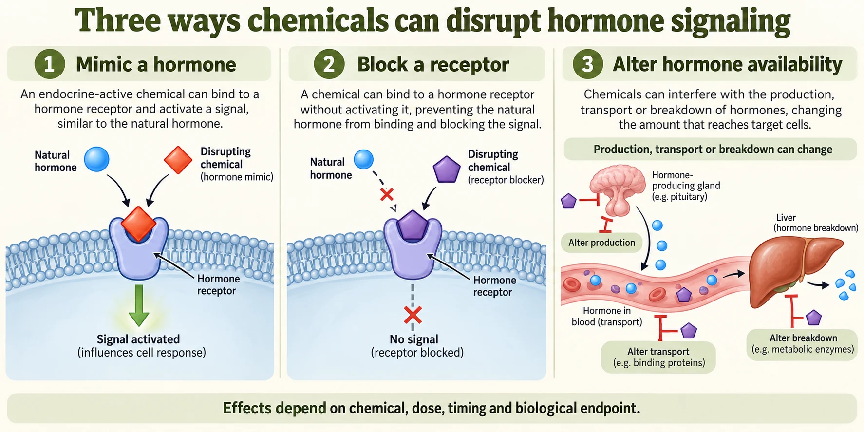
Endocrine-disrupting chemicals interfere with hormone production, transport, signaling or breakdown. Effects depend on the chemical, dose, route, exposure timing and endpoint. Some responses occur at low doses or are nonmonotonic, but neither property applies identically to every chemical or outcome.
Major Endocrine Disruptors
- BPA: Bisphenol A has been used in polycarbonate plastics and epoxy resins. Laboratory and human studies investigate hormone-related effects. Detection in a biomonitoring survey demonstrates exposure, not that the same percentage of people has a diagnosed effect.
- Phthalates: Some are plasticizers or ingredients in consumer products. Certain phthalates disrupt androgen-related development, often through anti-androgenic mechanisms; the group contains chemicals with different uses and hazards.
- DDT: A persistent organochlorine insecticide with endocrine-related effects that vary among isomers and metabolites. Many uses are prohibited or restricted, while the Stockholm Convention allows specified disease-vector-control uses under its requirements.
- PCBs: A family of industrial chemicals with congener-dependent persistence and biological effects, including disruption of thyroid and other signaling pathways. Legacy equipment and sediments remain exposure sources after production restrictions.
- Atrazine: A herbicide studied for effects on endocrine pathways and amphibian development. Results depend on species, life stage, exposure and experimental design; a single low concentration does not define a universal frog response or human risk threshold.
- Dioxins: Some dioxins and related compounds act through the aryl hydrocarbon receptor and can affect development, reproduction and other systems. Potency differs substantially among congeners; mixtures are often assessed using toxic-equivalency methods.
- Parabens: Preservatives used in some personal-care products. Certain members show estrogenic activity in experimental systems; potency, exposure and metabolism influence interpretation.
- Flame retardants: Some PBDEs and other substances have endocrine or developmental concerns. The category is chemically diverse, so findings for one compound cannot automatically be transferred to every flame retardant.
Mechanisms of Endocrine Disruption
- Mimicry (Agonist): Chemical structure similar to natural hormone (e.g., estrogen); binds hormone receptor; activates same signaling pathway; estrogenic effect at wrong time/place
- Blocking (Antagonist): Chemical binds receptor but doesn't activate; blocks natural hormone from binding; prevents normal signaling
- Synthesis Alteration: Interferes with hormone synthesis (e.g., inhibits enzyme); reduces circulating hormone levels; disrupts downstream effects
- Metabolism Changes: Increases hormone breakdown/excretion; reduces hormone availability/duration
- Receptor Expression: Alters number/sensitivity of hormone receptors; changes tissue responsiveness to hormones
- Generational effects: Developmental exposure can have lasting consequences, and research investigates epigenetic mechanisms. Direct exposure of a fetus and its developing germ cells differs from a demonstrated effect in an unexposed later generation.
Critical Windows of Exposure
- Prenatal development: Hormones coordinate organ development, creating sensitive exposure windows. A chemical’s effect depends on dose, timing and target system; small exposures do not inevitably cause major permanent injury.
- Infancy/Childhood: Continued development; thyroid hormone critical for brain development; disruption affects IQ, behavior
- Puberty: Reproductive system maturation; disruption affects fertility, sexual function
- Adulthood: Hormones continue to regulate reproduction, metabolism and other functions. Studies investigate links between particular exposures and disease; evidence and causal confidence differ among chemicals and outcomes.
- Dose-Timing Interaction: Same dose at different life stages has different impacts; developmental window determines severity
Health Effects in Humans and Wildlife
- Reproduction: Experimental and observational studies examine fertility, reproductive development, sperm measures and ovulation. Identify the chemical, species and exposure before generalizing an effect.
- Development: Some exposures can affect thyroid signaling and neurodevelopment. A statistical association with learning or behavior does not mean every exposed child will develop a specific disorder.
- Metabolism: Research examines altered appetite regulation, fat storage and glucose metabolism for certain endocrine-active compounds. Evidence varies by endpoint and study design; these are multifactorial health outcomes.
- Cancer: Some chemicals have established or suspected carcinogenic effects, including hormone-related mechanisms. Assess the specific substance and exposure rather than treating endocrine disruption as a uniform cancer diagnosis.
- Immune effects: Particular chemicals can alter immune development or function. These effects require substance-specific evidence and are not a defining property shared by every endocrine disruptor.
- Wildlife: Environmental estrogens can alter fish reproductive traits; DDE contributes to eggshell thinning in susceptible birds. Atrazine experiments illustrate the need to examine dose, species and replication rather than memorize one universal response concentration.
- Population consequences: Altered reproductive success can affect populations when exposure is sufficient and sustained. Individual biomarkers, fertility changes and ecosystem collapse are different levels of evidence.
- Human Evidence: Epidemiological links between BPA exposure and reproductive/metabolic effects; causation difficult to prove
Nonmonotonic Dose-Response
- Monotonic response: A response consistently increases or decreases across the tested dose range, although it need not be linear. Thresholds depend on endpoint and evidence; a lethal-dose test alone cannot establish a no-effect dose.
- Nonmonotonic response: The slope changes sign across the measured dose range, producing patterns such as U-shaped or inverted-U curves. This does not mean that the lowest dose always causes the greatest effect.
- Biological Reason: Receptor saturation; feedback loops; at very high doses, saturation/toxicity masking hormone-like effects
- Assessment challenge: Sensitive endpoints, relevant life stages and suitable dose spacing help detect effects missed by a narrow test design. measures lethality, while developmental and chronic studies answer different questions.
- Examples: Hormone and endocrine-active chemical experiments can show endpoint-specific nonmonotonic patterns. Read the actual curve and uncertainty; a simplified concentration pair cannot describe every atrazine or BPA study.
- Implication: High-dose results may not predict lower-dose responses when a relationship is nonmonotonic. Assessment therefore examines mechanism, exposure and evidence across relevant doses rather than assuming either universal safety or universal harm.
Exam tip: Connect mimicry, receptor blocking and altered hormone availability to a biological endpoint. Distinguish low-dose effects from nonmonotonicity, and direct multigenerational exposure from inherited effects in unexposed generations. Explain sensitive developmental windows without assuming every endocrine-active chemical has the same response.
8.4 Human Impacts on Wetlands and Mangroves
Wetland Characteristics and Value
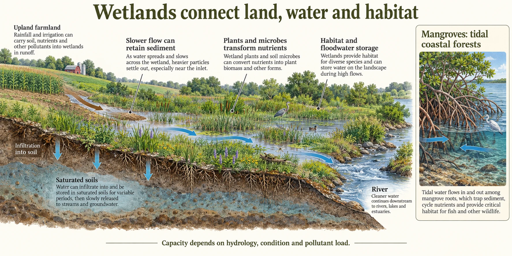
Wetlands have water at or near the surface for periods sufficient to shape soils and biological communities. Marshes, swamps, peatlands and tidal wetlands differ in hydrology and ecology. They support habitat, water storage, nutrient cycling and carbon stocks; their value depends on location and condition rather than one universal dollar value per hectare.
Wetland Types and Functions
- Freshwater Marshes: Herbaceous vegetation (reeds, cattails); high productivity; sediment/nutrient trapping; wildlife habitat
- Swamps: Woody vegetation (trees, shrubs); more structured; often forested wetlands (cypress swamps, bottomland hardwoods)
- Bogs: Acidic, nutrient-poor; sphagnum moss dominant; peat accumulation; carbon-rich; unique specialized species
- Fens: Peat-forming wetlands influenced by groundwater or mineral-rich surface water. They are generally less acidic and more mineral-rich than bogs, but not all fens are alkaline or share the same vegetation.
- Functions: Wetlands can store floodwater, slow flow, retain sediment, transform nutrients and support wildlife. Storage and treatment capacity are finite; some contaminants accumulate rather than being destroyed, and benefits depend on hydrology.
- Human benefits: Wetlands support fisheries nurseries, waterfowl, recreation and livelihoods. Dependence differs among species and regions; a fixed percentage of all commercial fish is not a universal wetland relationship.
- Carbon: Waterlogged soils can slow decomposition and store large carbon stocks, especially in peat. Draining or disturbing them can release carbon. Compare soil depth, ecosystem type and methane emissions when assessing climate benefits.
Wetland Loss and Causes
- Loss: The Global Wetland Outlook 2025 estimates about 411 million hectares, approximately 22% of the global total, lost since 1970. Other historical baselines yield different estimates. Extent loss and degradation of remaining wetlands are distinct measures.
- Causes: Agricultural conversion, urban filling, altered river flows, extraction and pollution affect different wetland types. Regional land-use evidence is needed to assign shares rather than a fixed global percentage breakdown.
- Agriculture: Drainage and filling change wetland hydrology and permit cultivation, while oxidation and subsidence can degrade organic soils. Initial crop benefits may be offset by lost water regulation, carbon storage and habitat.
- Urban Expansion: Wetlands filled for development; urban sprawl eliminates nearby wetland habitat
- Pollution/Eutrophication: Nutrient runoff changes species composition; invasives outcompete natives; ecosystem simplification
- Water Withdrawal: Dams, irrigation reduce wetland water levels; Aral Sea example: irrigation diversion desiccated sea, environmental catastrophe
- Legacy Effects: Even where protection established, wetland functions recover slowly; hydrologic regime restoration difficult
Mangrove Ecosystems
- Mangroves: Salt-tolerant trees and shrubs form tropical and subtropical intertidal forests. Adaptations vary among species and include salt exclusion or excretion and specialized roots in oxygen-poor soils.
- Distribution: Mangroves occur along suitable tropical and subtropical coasts in Asia, Africa, the Americas and Oceania. National inventories and satellite maps use different definitions; their area is far larger than an old four-million-hectare estimate.
- Value: Roots and forest structure can reduce waves, trap sediment, store carbon and provide nursery habitat. Protection depends on forest width, condition, water depth and storm characteristics; mangroves do not guarantee protection from every tsunami or cyclone.
- Pressures: Aquaculture, agriculture, urban development, wood extraction and altered sediment or tidal flows have caused losses. Trends and drivers vary by region, with restoration and natural expansion occurring in some places.
- Aquaculture trade-offs: Converting mangroves to ponds can generate income but remove habitat, carbon storage and coastal protection. Long-term outcomes depend on pond management, water quality, markets and alternative siting.
- Economic comparison: Compare locally measured restoration costs, sustained aquaculture income and the full range of ecosystem services over the same period. Fixed million-dollar-per-hectare figures are not transferable among projects.
- Climate Adaptation: Mangroves can migrate upland as seas rise (if space available); migration blocked by development (trapped)
- Restoration Efforts: Mangrove restoration projects accelerating; costs high; success variable (often fails if not addressing causes)
Exam tip: Link wetland hydrology to habitat, sediment retention, nutrient transformation and carbon storage. Compare benefits of conversion with lost services, including distribution of costs. Successful restoration addresses tidal or freshwater flow and the original cause of degradation, as well as planting.
8.5 Eutrophication
Process and Mechanism
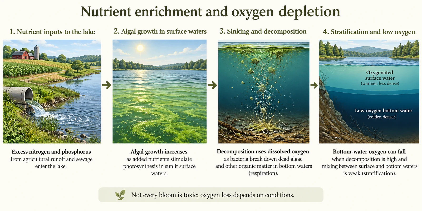
Eutrophication is nutrient enrichment of an aquatic ecosystem, often involving nitrogen and phosphorus. Excess loading can increase production, alter communities and contribute to oxygen depletion. Cultural eutrophication describes acceleration by human activities; it is not an inevitable identical aging sequence in every lake.
Eutrophication Cascade
- Nutrient Input: Agricultural runoff (fertilizers), sewage (human waste), atmospheric deposition, stormwater (urban); nitrogen/phosphorus concentrations increase
- Algal Bloom: Excess nutrients stimulate algae/cyanobacteria growth; population explosive; water turns green/murky
- Shading: Dense algal layer blocks sunlight; aquatic plants die (cannot photosynthesize)
- Decomposition: Microbial respiration consumes oxygen while breaking down organic matter. A simplified balanced aerobic reaction is . Algae also respire, and nighttime oxygen demand can matter before a bloom dies.
- Hypoxia: Dissolved oxygen below about 2 is a common operational definition in coastal studies. Species and life stages differ in tolerance; stress can occur above this value, depending on temperature and exposure duration.
- Anoxia: With little or no dissolved oxygen, anaerobic pathways become important. Methane or sulfide may form under suitable conditions, but their production depends on substrates and water chemistry.
- Fish Kills: Acute hypoxia causes massive fish mortality; sometimes visible (floating fish); ecosystem disruption
- Dead zones: Severe oxygen depletion excludes many aerobic organisms. These zones may be seasonal, intermittent or persistent; the name does not mean that all forms of life disappear.
Global Dead Zones
- Global observations: Hundreds of coastal systems have documented hypoxia. Inventories change with monitoring coverage and definitions; area, severity and duration provide more information than a single count.
- Examples: The northern Gulf of Mexico, Baltic Sea, Black Sea and Chesapeake Bay illustrate different oxygen-depletion settings. Annual mapped areas vary with runoff, weather, stratification and the survey method.
- Sources: Agricultural nutrients, wastewater, atmospheric nitrogen and other inputs contribute in different proportions. Control programs use watershed-specific nutrient budgets rather than a universal agricultural percentage.
- Gulf example: The Mississippi–Atchafalaya watershed delivers nutrients and freshwater to the northern Gulf. Nutrient-fueled production and density stratification contribute to summer bottom-water hypoxia; storms and seasonal mixing alter its extent.
- Baltic example: Nutrient inputs, restricted exchange, stratification and internal nutrient recycling contribute to oxygen problems. Their effects interact with fishing and other ecological pressures rather than explaining every catch trend alone.
- Economic effects: Low oxygen and harmful blooms can displace fish, alter catches, close shellfish harvests, impair tourism and raise treatment costs. Impacts vary among locations and years; they do not imply every affected fishery has collapsed.
- Trends: Nutrient loading and warming can increase risk through production, stratification and lower oxygen solubility. Local controls can improve conditions, so expanding hypoxia is a risk rather than an inevitable trajectory everywhere.
Harmful Algal Blooms (HABs)
- Definition: Dense algal growth; some species produce toxins; public health concern; distinct from benign algal blooms
- Toxin producers: Some cyanobacteria produce microcystins or anatoxins. Certain dinoflagellates produce saxitoxins; domoic acid is associated with some Pseudo-nitzschia diatoms. Toxin production differs among species and strains.
- Human Health: Drinking water contamination causes neurological/hepatological effects; shellfish poisoning (bioaccumulation in clams, mussels)
- Bloom conditions: Nutrients, temperature, water residence time, circulation and species composition influence blooms. Better monitoring also changes reported counts; not every increase in reports measures the same ecological change.
- Red tides: Some harmful marine blooms discolor water, but harmful blooms may be colorless and colored blooms may be harmless. Different organisms cause different toxins and effects; red coloration does not identify a single poisoning syndrome.
- Economic Disruption: Shellfish harvesting closures; fishing restrictions; water treatment challenges
- Prevention and exposure control: Reduce relevant nutrient sources, monitor toxins and follow local water or harvest advisories. Drinking-water treatment must address the specific organism and toxin; killing cells alone does not guarantee removal of released toxins.
Solutions and Recovery
- Nutrient Reduction: Source control most effective; fertilizer best management practices (reduce application, timing, placement); wastewater treatment (secondary + tertiary); sewage nutrient removal
- Farm practices: Soil testing, appropriate fertilizer rates and timing, cover crops, erosion control and riparian buffers can reduce losses. Performance depends on soil, weather and whether nutrients move attached to sediment or dissolved in water.
- Wetlands: Wetland plants and microbes can retain nutrients and convert nitrate to nitrogen gas through denitrification. Capacity depends on residence time and loading; restoring a wetland does not instantly reproduce every lost function.
- Urban Stormwater: Green infrastructure (rain gardens, permeable pavement, bioswales) traps/filters runoff; reduces nutrient loading
- Recovery: Stored sediment phosphorus and continuing watershed inputs can sustain enrichment after external loads decline. Recovery times differ among systems, and water chemistry can improve before biological communities fully recover.
- Case studies: Lake Erie and Chesapeake Bay show both benefits of nutrient controls and continuing challenges. Legacy nutrients, agricultural runoff, weather and warming can complicate or reverse earlier gains.
- Limitation: Phosphorus often limits freshwater production and nitrogen often limits coastal marine production, but co-limitation and exceptions are common. Use ecosystem evidence to select controls; addressing both nutrients may be necessary.
- Challenge: Political/economic resistance to agricultural changes; fertilizer subsidies encourage high use; tragedy of commons (individual farmers don't control downstream effects)
Exam tip: Explain nutrient enrichment, increased production, respiration and decomposition, and reduced oxygen replenishment. Distinguish hypoxia from algal toxicity. Compare point and diffuse controls, and explain why internal nutrient recycling and ecological recovery can delay improvement after source reductions.
Worked example: oxygen demand in a diluted BOD bottle
In a simplified unseeded five-day BOD test, a diluted bottle starts at 8.5 dissolved oxygen and finishes at 4.5 . The original sample is 2% of the bottle volume, so its dilution fraction P is 0.02.
This estimates oxygen consumed under the test conditions, not the water’s initial dissolved-oxygen concentration. Real methods specify temperature, blank checks, valid depletion, seed corrections where relevant and whether nitrification is included or suppressed. is not necessarily all ultimate oxygen demand.
8.6 Thermal Pollution
Sources and Temperature Effects
Thermal pollution is a human-caused change in a water body’s temperature regime. Warm discharges are common examples, but unusually cold dam releases and abrupt temperature shifts can also disrupt aquatic life.
Primary Sources
- Power-plant cooling: Once-through cooling withdraws water and returns it warmer; recirculating systems have different withdrawal and consumption patterns. Temperature increases and national water-use shares depend on technology, operating conditions and the reporting year.
- Industrial Cooling: Steel mills, paper mills, petrochemical plants discharge hot water; concentrated thermal pollution
- Dam Operations: Large dams release cool deep water (or warm surface water depending on operation); alters natural thermal regime
- Urban Heat Island: Stormwater runoff heated by impervious surfaces (pavement, roofs); contributes warming downstream
- Climate Change: Background warming + anthropogenic thermal pollution combine; synergistic stress on cold-water species
- Combined stress: An added thermal load can push sensitive organisms beyond favorable conditions, especially during low flow or heat waves. Actual effects depend on species, acclimation, oxygen and the timing and spatial extent of exposure.
Biological Effects
- Tolerance: Species have different thermal optima and limits, which vary with life stage, acclimation and exposure duration. A trout optimum is not a universal lethal threshold, and “warm-water fish” is not one temperature category.
- Metabolism: describes how a measured biological rate changes over a 10 °C interval. A value of two is an illustrative approximation for some processes within suitable ranges, not a law applying at all temperatures.
- Double Stress: Warm-water discharge increases demand while decreasing availability (solubility); fish suffocation risk even if not directly lethal temperature
- Migration/Spawning Disruption: Salmon use temperature cues for migration timing; abnormal temperatures confuse populations; reduced spawning success
- Community change: Warmer conditions can favor heat-tolerant species and disadvantage cold-water specialists. Responses depend on oxygen, habitat and interactions; avoid assuming every replacement species has the same ecological role.
- Algae: Temperature can favor some algae or cyanobacteria, but light, nutrients, grazing and flow also control growth. Heating does not independently create unlimited algal production.
- Disease: Thermal stress and temperature-dependent pathogen or parasite growth can alter disease risk. The relationship varies among organisms; not every parasite benefits from warmer water.
- Invertebrate Impacts: Mayflies, caddisflies temperature-sensitive; loss cascades through food web; reduced food for fish/birds
Thermal Stratification and Mixing
- Thermal Stratification: Water layers by temperature/density; warm water surface (epilimnion), cool bottom (hypolimnion), transition (thermocline)
- Stratification: Warm surface inputs may strengthen density differences and reduce vertical exchange under suitable conditions. Plume mixing, depth, wind and freshwater or salt gradients determine the actual response.
- Dam releases: Deep releases may be cold and oxygen-poor, while surface releases can be warmer. Selective withdrawal and aeration can help manage downstream temperature and oxygen; cold releases do not automatically suppress eutrophication beneficially.
- Nutrient cycling: Reduced mixing can limit exchange between surface and deep water, while oxygen depletion can increase sediment phosphorus release. Productivity and nutrient availability may therefore change in different directions.
- Complexity: Thermal effects intertwine with nutrient cycling, oxygen dynamics; ecosystem responses multifaceted
Mitigation and Climate Change Interaction
- Cooling Technologies: Cooling towers evaporatively cool; natural draft towers (tall, passive); mechanical (fans, expensive); wet/dry hybrids
- Recirculation: Established recirculating cooling systems reduce withdrawals relative to once-through cooling, but evaporative systems can consume more water. Compare withdrawals, consumption, energy use and heat rejection separately.
- Heat management: Cooling towers, ponds or heat reuse can reduce the thermal load reaching a receiving water. A mixing zone dilutes a plume but does not destroy its heat or replace compliance with applicable temperature limits.
- Timing/Location Restrictions: Seasonal discharge limits (avoid spawning); location away from nurseries; regulatory approach
- Warming interaction: Climate warming and heated discharges can compound stress on cold-water habitat. Riparian shading, flow management and source controls can reduce local pressures, although their effectiveness is site-specific.
- Energy choices: Wind and photovoltaic electricity avoid operational steam-cycle cooling, while other energy technologies have different water and heat demands. Plant retrofits, cooling changes and discharge management also provide mitigation options.
- Regulation: Permits and water-quality requirements can address temperature and cooling impacts. Assess the jurisdiction and receiving-water objectives; thermal controls are not universally vague or unenforceable.
Exam tip: Explain the double stress of increased biological oxygen demand and lower oxygen solubility in warmer water. Include cold dam releases, thermal shock and species-specific tolerances. Compare cooling options by withdrawal, consumption, heat rejection and energy demand; interpret only over a stated interval.
Worked examples: mixing temperature and
Assume equal water density and heat capacity, complete mixing, and negligible heat exchange with surroundings. A stream at 10 and 15 °C mixes with an outfall at 2 and 30 °C.
The result describes an ideal mixed temperature, not an entire downstream plume or a permit determination. Now suppose a measured process has of two within the relevant temperature range.
A 5 °C increase gives about a 41% rate increase under this model. Outside the tested range, stress, enzyme limits and acclimation can invalidate the approximation; it is not a universal fish-metabolism forecast.
8.7 Persistent Organic Pollutants (POPs)
Definition and Characteristics
Persistent organic pollutants resist degradation, can be transported over long distances and can accumulate in organisms, producing harmful effects. Many classic chlorinated POPs associate with lipids, while some newer listed substances bind differently, including to proteins. Persistence and uptake depend on compound and environment.
Key Characteristics
- Persistence: Chemical structure can resist biological, chemical or photochemical breakdown. Half-lives differ among air, soil, sediment and organisms; persistence is not explained by carbon–carbon bonds alone or one universal lifetime.
- Partitioning: Many legacy POPs favor organic matter and lipids and are eliminated slowly. Some PFAS associate with proteins and other compartments. Slow elimination differs from being impossible to metabolize or excrete.
- Accumulation: Tissue concentrations reflect uptake, elimination, metabolism and growth dilution. Factors vary with organism, tissue and measurement basis; every POP does not share a fixed factor above one thousand.
- Atmospheric transport: Some semivolatile compounds repeatedly exchange between air and surfaces and travel far before degradation. Particle-bound transport also matters. Volatility and weather determine the pathway and distance.
- Low Volatility POPs: Less volatile compounds transported via ocean currents; attach to particles; settle to sediments; remobilize; persistent multi-decade timescale
- Widespread detection: POPs have been measured far from sources, including polar ecosystems and human tissues. Detection establishes presence; concentration, exposure and toxicology determine the significance of a particular result.
Major POPs and Sources
Pesticides - DDT and HCHs
- DDT: An insecticide used in agriculture and vector control, prohibited for most US uses in 1972. The Stockholm Convention restricts its use and allows specified disease-vector control subject to requirements; permitted uses and inventories change over time.
- Persistence: DDT and its metabolites can remain in soils, sediments and food webs after use ends. Rates vary with temperature, oxygen, organisms and chemical form, so environmental and biological half-lives should be distinguished.
- Health Effects: Probable carcinogen; endocrine disruptor (estrogenic); reproductive effects; neurodevelopmental impacts; nervous system damage
- Wildlife: DDE, a DDT breakdown product, contributes to eggshell thinning and reproductive failure in susceptible birds. Reduced exposure, habitat protection and other conservation actions supported raptor recovery; responses varied among regions and species.
- HCHs: Hexachlorocyclohexanes include different isomers; lindane is the gamma isomer formerly used as an insecticide and in some pharmaceutical applications. Persistence, transport and toxicity differ among isomers.
- Current management: Treaty restrictions, exemptions, stockpiles and contaminated sites determine continuing releases. DDT and certain HCHs are covered through different listings; a country’s economic category alone does not establish its current use.
Industrial Chemicals - PCBs
- PCBs: Polychlorinated biphenyls comprise 209 possible congeners. Their electrical-insulating and heat-transfer properties led to use in transformers, capacitors and other equipment. Production restrictions do not remove chemicals remaining in equipment or sediments.
- Persistence: PCB behavior varies with chlorine substitution, environmental medium and metabolism. Some congeners persist for long periods, but they do not all have the same half-life or the highest accumulation of every organochlorine.
- Effects: PCBs can affect immune, reproductive, neurological and other functions. Carcinogenicity assessments and dioxin-like activity depend on the evidence and congener profile; mixtures need more than one generic potency label.
- Hudson River: Legacy industrial PCB discharges contaminated river sediments and fish, leading to Superfund remediation and continuing management. Dredging, monitoring and fish advisories address different parts of the exposure pathway.
- Legacy stocks: PCB-containing equipment and waste require identification, safe management and destruction. Distinguish pure PCB mass from the much larger mass of equipment or contaminated material containing it; these inventories are not interchangeable.
- Fish advisories: Local monitoring supports advice for particular waters, species and populations. An advisory can remain relevant after discharges stop because sediment and food-web exposure persist; use current local guidance.
Combustion Byproducts - Dioxins and Furans
- Dioxins and furans: Chlorinated dibenzo-p-dioxins and dibenzofurans can form unintentionally in some combustion and industrial processes. Their many congeners differ in toxicity; selected dioxin-like compounds are assessed using toxic-equivalency approaches.
- TCDD: A potent dioxin congener with marked species differences in acute toxicity. Acute values and chronic reference doses describe different endpoints and exposure durations; they cannot be substituted for one another.
- Furans (PCDFs): Similar to dioxins; also combustion byproducts; similar toxicity/persistence; often co-emitted with dioxins
- Persistence: WHO describes human dioxin half-lives around 7–11 years, with variation among congeners and individuals. Environmental persistence and food-web accumulation depend on the medium and chemical form.
- Effects: Dioxin exposure can affect development, reproduction, immunity and other systems. TCDD is classified as carcinogenic to humans; this classification does not assign identical potency to every dioxin or furan.
- Seveso: The 1976 industrial accident in Italy released TCDD and contaminated surrounding communities and land. Long-term health follow-up illustrates persistent exposure concerns; release estimates and affected-population counts depend on the investigation.
- Sources and controls: Poorly controlled burning, metal processing and some chemical processes can release dioxins. Cleaner processes, combustion control, rapid gas cooling and appropriate emission treatment reduce releases; dominant sources vary by region.
Global Transport and Arctic Concern
Grasshopper Effect
- Grasshopper effect: Repeated volatilization, transport and deposition can move semivolatile POPs across regions. Cooler conditions can favor deposition and retention, but the pathway depends on volatility, degradation and circulation.
- Temperature effects: Temperature changes air–surface partitioning, supporting repeated exchanges along a transport pathway. The mechanism is not a guaranteed sequence from equator to tropics to pole for every pollutant.
- Polar accumulation: Cold regions can retain transported contaminants, but they are not irreversible final sinks. Chemicals can re-enter air or water as conditions change, and local as well as remote sources may contribute.
- Seasonal cycling: Warming and cooling alter exchanges between air, snow, soil and water. Wind, ocean circulation and chemical properties determine transport direction; seasonal exchange is not limited to a fixed latitude range.
- Distance from Source: POPs found everywhere globally; POPs measured in Arctic despite application thousands of km away; demonstrates atmospheric persistence/transport
- Climate Change Impact: Warming reduces temperature gradient; may alter transport patterns; could mobilize stored Arctic POPs (permafrost thaw)
Arctic Populations and Bioaccumulation
- Arctic exposure: Some Indigenous communities face elevated exposure to particular contaminants through locally important foods. Levels vary among places, species and diets; there is no universal ranking or multiplier for all Inuit populations.
- Early-life transfer: Some contaminants cross the placenta or enter human milk. Biomonitoring informs prevention at the source; feeding decisions should follow current public-health advice and account for the substantial benefits of breastfeeding.
- Health evidence: Arctic studies investigate contaminant mixtures alongside nutrition, social conditions and other exposures. Associations, mechanisms and causal conclusions differ by outcome; community-specific evidence is essential.
- Traditional Food Importance: Inuit rely on traditional foods for cultural identity, nutrition, independence; removing foods stigmatizes culture; health/cultural compromise
- Treaty recognition: The Stockholm Convention recognizes particular risks to Arctic ecosystems and Indigenous communities. Implementation involves national plans, technical assistance, monitoring and financing as well as chemical restrictions.
- Environmental Justice Issue: Arctic residents exposed to chemicals from distant sources; no input into use decisions; bearing health burden from global industrialization
Stockholm Convention and Remediation
International Regulation
- Convention: Adopted in 2001 and in force from 2004, the Stockholm Convention addresses elimination, restriction and unintentional releases through different annexes. Its chemical listings have expanded; a dated listing and ratification status are needed for exact totals.
- Initial twelve: Aldrin, chlordane, DDT, dieldrin, endrin, heptachlor, hexachlorobenzene, mirex, toxaphene, PCBs, dioxins and furans. HCHs were later additions, not replacements for dieldrin in the original list.
- Later Additions: Brominated flame retardants (PBDEs), perfluorinated compounds (PFOA, PFOS), endosulfan; newer POPs identified with increasing knowledge
- Obligations: Parties implement the relevant annex requirements for production, use, stockpiles, waste and releases, subject to treaty provisions. Being a signatory and becoming a party are different legal steps.
- Exemptions: Some countries exempt for specific uses (DDT for malaria control); creates controversy (needed for disease control vs. health/environmental risk)
- Enforcement Challenge: No supranational enforcement authority; relies on national implementation; developing nations often lack resources; progress variable
Remediation and Cleanup
- Sites: Cleanup scope, cost and duration depend on contaminant, volume, exposure pathways and available technology. Investigation and risk-based prioritization precede selecting treatment; one cost range cannot cover all sites.
- Remediation Methods: Incineration (high-temp destruction, expensive), soil excavation + treatment, dredging (remove contaminated sediments), capping (seal contamination in place, not removal)
- Dredging trade-offs: Removing contaminated sediment can reduce future exposure but may temporarily resuspend material and creates waste for treatment or disposal. Capping, source control and monitoring may form part of a site-specific remedy.
- Residuals: Treatment can destroy or isolate contaminants, but verification and long-term management may remain necessary. Persistent does not mean indestructible, and excavation alone transfers rather than destroys contaminated material.
- Preventing New Contamination: Most cost-effective approach; eliminate POP production/use; proper waste management (prevent incineration emissions)
- Challenge: Developing nations lack remediation resources; contaminated sites pose ongoing exposure; legacy burden from developed nation industrialization
Exam tip: Connect persistence, transport, partitioning and slow elimination to exposure. Distinguish classic lipid-associated POPs from compounds with other binding behavior. Explain DDT/DDE, PCBs and dioxins using their sources and effects, and compare source prevention, destruction, removal and containment.
8.8 Bioaccumulation and Biomagnification
Concepts and Mechanisms
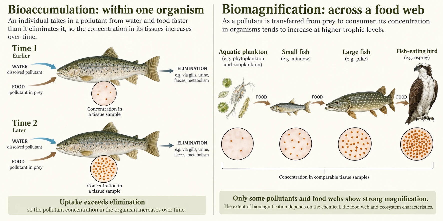
Bioaccumulation describes chemical uptake from all exposure routes in an organism over time. Biomagnification is increasing concentration between prey and consumers or across trophic levels. These processes depend on chemical and food-web properties; neither occurs by a fixed factor in every ecosystem.
Bioaccumulation Mechanics
- Storage: Some persistent organic chemicals partition into lipids; others bind proteins or other tissues. Metabolism and excretion can occur, but uptake may exceed removal. Growth dilution and changes in body composition also affect concentration.
- BAF:. An aquatic tissue-to-water factor commonly has units of when tissue is measured in and water in . State wet-weight or lipid basis and exposure conditions. A bioconcentration factor isolates uptake from water, whereas a BAF includes all routes.
- Steady state: Body burden can approach balance when uptake equals elimination under stable conditions. Tissue concentration also depends on growth and distribution; changing exposure can prevent a steady state from being reached.
- Elimination: Biological half-life depends on chemical form, species, tissue, age and exposure history. A human elimination estimate cannot automatically be applied to a fish, or to a different PCB or PFAS.
- Age: Longer exposure can increase burdens of slowly eliminated compounds, but changing diets, environmental concentrations, growth and metabolism alter trends. Older individuals do not always have the highest concentration of every contaminant.
- Exposure routes: Food is important for several classic POPs, while water, dust, air or occupation can dominate for other compounds and settings. Specify the chemical and population before assigning an exposure-route percentage.
- Physiology: Body composition, diet, metabolism and reproductive transfer can affect burdens. Lactation may transfer some contaminants, but a fixed percentage of maternal load does not describe all substances or families.
Biomagnification Through Food Chains
- Trophic transfer: Consumers ingest contaminated prey. Magnification is possible when assimilation is high relative to elimination, metabolism and growth dilution; the predator still has removal processes.
- BMF:. Concentrations must use comparable tissue or whole-body and normalization bases. A ratio above one supports magnification for that comparison; five- or ten-fold increases per level are not universal.
- Illustrative sequence: If comparable tissue concentrations rise from 10 to 100 to 1,000 to 10,000 units through successive consumers, the last is 1,000 times the first. A water value of one in a genuinely comparable concentration basis would make the last 10,000-fold higher, not ten million-fold. Real tissue-to-water comparisons usually require explicit unit conversion.
- Mercury: Microorganisms can transform inorganic mercury into methylmercury, which can accumulate and magnify in aquatic food webs. Coal combustion is one source among natural and human sources; chemical speciation is crucial.
- Chemical differences: Persistence and slow elimination favor magnification but do not guarantee it. Methylmercury magnifies strongly, while many other metals are regulated, transformed or behave differently. Degradable pesticides can still cause toxicity without biomagnifying.
- Changing exposure: Continued contaminated feeding can sustain a burden. Reducing exposure may permit depuration, although slow elimination, ongoing sources and sediment reservoirs can delay the decline.
- Food-web context: Magnification occurs in both aquatic and terrestrial systems. Food-chain length, metabolism, diet and chemical partitioning matter; a universal aquatic–terrestrial ranking based only on trophic efficiency is unreliable.
Top Predators at Risk
- Raptors: DDE exposure contributed to eggshell thinning and reproductive failure in susceptible birds, including bald eagles and peregrine falcons. Restrictions and conservation helped recovery, with different timelines among populations.
- Eggshell mechanism: DDE can interfere with normal shell formation, causing thinner shells that break more readily. Severity varies with species and exposure; a fixed 20% reduction and zero hatching are not universal outcomes.
- Marine mammals: Some long-lived predators accumulate substantial PCB burdens. Studies examine reproductive and immune effects, but concentrations and outcomes differ among species and populations; a single ppm value is not representative.
- Large Fish: Sharks, swordfish, tuna accumulate high mercury; consumption advisories for pregnant women, children (neurological risk)
- Long-lived species: Extended exposure and slow elimination can increase body burdens, but age alone does not determine concentration. Slow reproduction can delay population recovery; generation time varies widely among species.
- Population-Level Effects: High concentrations can impair entire populations; reproductive failure cascades; local extinctions possible; ecosystem disruption
Human Exposure and Dietary Choices
- Human diets: Exposure depends on the contaminant and food source, not merely whether someone is vegetarian or pescatarian. Trophic level, location, feed contamination and portion patterns influence exposure; foods also provide nutritional benefits.
- Advisories: Follow current local fish advisories and relevant national guidance for species, water body and population. Commercial-fish advice and advisories for locally caught fish can use different evidence and purposes.
- Mercury in fish: Large predatory species often contain more methylmercury than short-lived lower-trophic species, but levels vary. There is no universal two-ppm boundary defining every meal as safe or hazardous; use current species-specific advice.
- PCBs in fish: Contaminated sediments and feeds can affect wild or farmed fish. Local monitoring and tissue preparation guidance matter; neither production method guarantees lower concentrations in all cases.
- Human biomonitoring: Results depend on the chemical, tissue, lipid adjustment, detection method, population and year. A generic human-milk concentration range is not a valid comparison across all POPs or all Arctic communities.
- Placental transfer: Some contaminants can cross the placenta. Maternal exposure, chemical properties and physiology determine transfer; a first child does not simply receive all of a mother’s accumulated load.
- Breastfeeding context: Source reduction and public-health monitoring reduce exposure while preserving the benefits of breastfeeding. Individual feeding decisions require current professional guidance rather than inference from a generic POP concentration.
Recovery Timeline and Persistence
- Depuration: With first-order removal and no further uptake, one, two and three half-lives leave 50%, 25% and 12.5% of the initial amount. Real elimination can involve several compartments, changing rates and continued exposure.
- Organism Replacement: Population recovery also depends on population turnover; slow-reproducing species (eagles, whales) take decades to recover even with individual depuration
- Recovery: US DDT restrictions, habitat measures and other protections supported substantial bald-eagle and peregrine-falcon recovery. National conservation status, local abundance and complete contaminant removal are different outcomes.
- Remobilization Risk: POPs stored in sediments; climate warming can cause re-volatilization; permafrost thaw releases legacy POPs; Arctic warming may cause "release" of accumulated POPs
- Prevention and recovery: Stopping exposure is important and can allow burdens to decline. Some effects may be irreversible while other organisms and populations recover; prevention is not the same as claiming accumulation can never decrease.
- Monitoring: Trends differ by compound, site and tissue. Declines following restrictions can coexist with persistent reservoirs and concern about replacement chemicals; current monitoring is needed before assigning a rising or falling trend.
Exam tip: Distinguish change within an organism from concentration differences across feeding relationships. Define BAF, BCF and BMF, including units and tissue basis. Explain uptake, transformation, elimination and growth dilution, and avoid assuming all persistent chemicals or metals magnify identically.
Worked examples: accumulation factors and half-life
Aquatic BAF: Let a fish have a measured whole-body wet-weight concentration of 2 and its surrounding water 0.001 , under specified exposure conditions.
Matched predator–prey BMF: If comparable tissue concentrations are 4 in a predator and 0.5 in prey, the unit cancels.
First-order depuration: With no further uptake, constant elimination rate and no changing body-mass effect, the remaining fraction after n half-lives is:
Three half-lives remove 87.5% under this simplified model. Real tissue concentrations may follow multiple compartments and continuing exposure; chemical depuration and ecological population recovery are separate processes.
8.9 Solid Waste Disposal
Overview and Scale
Municipal solid waste includes discarded household and similar commercial materials; industrial, construction and hazardous wastes may be counted separately. UNEP’s 2024 outlook estimates 2.1 billion tonnes of municipal waste generated globally in 2023. Collection, recycling, composting, combustion and disposal shares differ among countries and datasets.
Landfill Management
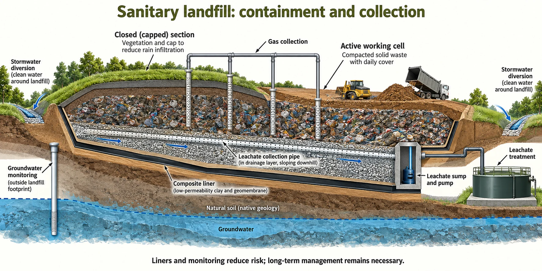
- Design: Sanitary landfills use compacted cells, cover, composite liners, leachate collection, gas controls and monitoring. Liners reduce leakage rather than being perfectly impermeable forever; design and operating requirements depend on the waste and jurisdiction.
- Leachate: Water moving through waste dissolves or carries organic compounds, ammonia, salts, metals and other material. Composition and pH change as a landfill ages; young acidic leachate and mature methanogenic leachate can differ greatly.
- Strength: Leachate may have high oxygen demand, ammonia and dissolved contaminants. Concentrations vary by waste, rainfall and age; BOD, COD and biodegradability must be measured rather than inferred from one generic range.
- Groundwater: Leachate escaping containment can migrate with groundwater flow and affect downgradient receptors. “Downwind” describes air transport, not groundwater movement. Monitoring, collection and treatment are selected for the actual contaminants and hydrogeology.
- Landfill gas: Anaerobic decomposition of biodegradable waste produces methane and , often in broadly similar proportions, with trace gases. Generation, collection efficiency and energy use vary with waste, moisture, age and infrastructure.
- Methane: Uncaptured gas contributes to warming and can create migration or safety hazards. Collection with flaring or energy recovery oxidizes methane to , reducing its climate effect, but capture is incomplete and combustion is not zero emissions.
- Capacity: Available airspace, waste density, diversion, settlement and permitted limits determine landfill lifetime. Regional capacity and hauling needs vary; a fixed twenty- or thirty-year lifespan is not universal.
- After closure: Gas and leachate generation, settlement, cap integrity and groundwater require continuing care. Monitoring duration and cleanup needs follow site conditions and rules; neither zero future risk nor a universal century-long cleanup can be assumed.
Incineration
- Combustion: Controlled burning reduces waste volume substantially and mass by a smaller proportion, leaving bottom ash and air-pollution-control residues. Volume and mass reductions are different measures; both depend on feedstock and process.
- Energy: Heat can produce steam for electricity and, in combined heat-and-power systems, useful district or industrial heat. Total useful-energy efficiency differs from electricity-only efficiency; recovery depends on a reliable heat demand.
- Emissions Problems: Burn creates air pollutants: dioxins/furans (POP formation, toxic), HCl (acid rain precursor), heavy metals (lead, mercury, cadmium), (smog), particulates
- Emission controls: Acid-gas scrubbers, particle collectors, activated-carbon injection and nitrogen-oxide controls address different pollutants. Performance depends on design, maintenance and operating conditions; captured contaminants remain in residues that need management.
- Ash: Bottom ash and finer captured residues have different contaminant profiles. Testing and applicable rules determine reuse, treatment or disposal; not all bottom ash is harmless, and not all jurisdictions classify every residue identically.
- Dioxin control: Dioxins can form during incomplete combustion or as gases cool in the presence of suitable precursors and surfaces. Good combustion, controlled cooling and gas treatment reduce formation and releases; temperature alone is not the entire control strategy.
- Controversy: Environmental justice concerns (incinerators often sited in low-income communities); air pollution disproportionately affects nearby residents; NIMBY resistance in wealthy areas
- Deployment: Waste combustion and energy recovery vary by region, waste policy and infrastructure. Facility counts change over time and differ for municipal, hazardous and other waste; compare like-for-like dated inventories.
Recycling and Composting
- US example:EPA’s 2018 municipal-waste dataset reports about 32.1% recycled and composted together, with recycling alone about 23.6%. These historical values are not current global rates; energy recovery and other food-management pathways are reported separately.
- Aluminium: Recycling generally saves substantial energy compared with producing primary metal from ore. Actual savings and collection rates depend on process and region; compare the same system boundary and data year.
- Plastics: Resin type, additives, sorting, contamination and markets determine recyclability. Mechanical recycling can degrade properties; chemical recycling has process-specific yields, energy needs and emissions. Collection does not guarantee recycling into a comparable new product.
- Economics Challenge: Recycling costs energy/labor; virgin material often cheaper (especially when energy abundant); market depends on material value; commodity price fluctuations affect viability
- Contamination Issue: Contaminated materials reduce quality; food-soiled cardboard, plastic with adhesives; require removal = labor-intensive; sorting infrastructure needed
- Composting: Food scraps, yard material and appropriate other organics can be processed into compost. Accepted feedstocks depend on the facility; coated or contaminated paper and “compostable” packaging are not universally accepted.
- Benefits: Well-managed compost can improve soil structure and recycle nutrients while diverting organics from anaerobic landfill decomposition. Aeration, moisture and feedstock control limit methane, odors and other emissions; benefits are not automatic for a poorly managed pile.
- Limitation: Recycling not infinitely scalable; contamination limits recycling; energy costs sometimes exceed environmental benefit; source reduction more effective
Global Disparities and Ocean Plastic
- Service gaps: Inadequate collection, controlled disposal and treatment can lead to open dumping and burning. Access differs within as well as among countries; define the service and population before assigning a global number.
- Waste trade: Some exported material is legitimately recovered, while misdeclared or poorly managed shipments can transfer pollution burdens. Traceability, informed consent and enforcement under applicable waste-trade rules matter.
- Plastic leakage: Mismanaged waste, stormwater, rivers, fishing activities and other pathways introduce plastics to waters. Estimates depend on whether they cover rivers, all aquatic environments or oceans; dated totals with different boundaries should not be mixed.
- Accumulation zones: Ocean circulation concentrates floating debris across broad, shifting areas. These are not solid garbage islands. Large debris fragments into smaller particles, while sinking, beaching and transport redistribute material.
- Justice: Coastal communities can bear cleanup, livelihood and ecosystem costs from locally generated and transported waste. Responsibility and exposure are shared unevenly; affected countries are not uniformly only receivers or only producers.
- Solutions Emerging: Single-use plastic bans; reusable alternatives; improved waste infrastructure; cleanup efforts (limited effectiveness); prevention critical
Exam tip: Compare source prevention, recovery and disposal using material flows. Trace leachate to groundwater and landfill gas to air; explain containment and long-term care. Distinguish incinerator mass from volume reduction, electricity efficiency from useful-heat recovery, and collection from successful recycling.
Worked example: disposal capacity
A hypothetical remaining landfill airspace is 120,000 . At an assumed compacted waste density of 0.60 tonnes per cubic meter and an incoming disposal rate of 60 tonnes per day:
This simple estimate ignores daily cover, settlement, changing diversion and operational limits. State whether the available volume is gross airspace or net waste airspace before applying a density.
8.10 Waste Reduction Methods
Waste Hierarchy
Waste hierarchy: Prevention and reuse generally precede recycling or composting, then energy recovery and disposal. Composting is a form of organic-material recovery, not always a lower rank than every recycling process. Product-specific life-cycle evidence helps evaluate trade-offs.
Source Reduction (Prevention)
- Consumer Behavior: Buy less; avoid unnecessary purchases; choose minimal packaging; decline single-use items; most effective but requires behavior change
- Durable design: Longer-lived, repairable products can reduce replacement demand. Benefits depend on actual use, maintenance and whether keeping an inefficient older product creates larger operating impacts.
- Packaging Reduction: Lighter packaging (uses less material), concentrated products (smaller volume), reusable containers; industry innovation ongoing
- Business Efficiency: Lean manufacturing reduces material waste; process optimization; waste elimination strategies; cost savings incentivize adoption
- Prevention potential: Material-efficient design, procurement and operations can avoid waste and disposal costs. Achievable savings depend on the starting process, product and service; no single percentage applies to all waste streams.
- Cultural Barrier: Consumerism promotes consumption; "throwaway culture" entrenched; sustainability values growing but minority; systemic change needed
Reuse and Repair
- Reuse: Repair, refurbishment, resale and sharing can extend useful life and displace new production. Actual resource savings depend on the displaced product, additional transport and how much longer the item is used.
- Containers: Reuse can reduce single-use packaging when items complete enough trips. Manufacturing material, washing, transport, losses and the local energy mix determine the break-even point.
- Right to Repair Movement: Challenge manufacturers' planned obsolescence; enable consumer/third-party repairs; longer product lifespan; reduced replacement need; economic + environmental benefit
- Repair Services Growth: Emerging repair cafes (community repair events); online tutorials enabling DIY repair; cultural shift toward fixing vs. replacing
- Donation/Redistribution: Reuse centers collect used items; distribute to need; extends product life; reduces new production demand; community benefit
- Constraints: Access to parts, information, safe design, skilled repair and cost influence repairability. Electronics and batteries are not inherently all unrepairable; safety requirements and specialist handling still matter.
Extended Producer Responsibility (EPR)
- Concept: Manufacturers responsible for end-of-life; incentivizes design for recyclability/reuse; cost internalization (includes disposal in price)
- Implementation: Take-back programs (return product at end-of-life); producer funds recycling; collection/processing infrastructure required
- Examples: Electronics (computers, phones); appliances; batteries; packaging (Germany, France); growing globally; automotive industry (vehicles, parts)
- EPR outcomes: Producer responsibility can fund collection and encourage better design when fees, standards and enforcement align with those goals. A take-back obligation alone does not guarantee longer life or lower hazardous content.
- Reverse Logistics: Complex supply chains for collection/processing; coordination with retailers/consumers; cost-intensive but feasible
- Challenges: Implementation costs; consumer participation required; enforcement variable; developing nations lack infrastructure
Container Deposits and Plastic Reduction
- Deposits: Refundable deposits create incentives to return covered containers. Return rate, collection rate and actual recycling yield are different measures; performance depends on deposit value, convenience, coverage and enforcement.
- Examples: Germany, Denmark, the Netherlands and several US states operate container-return systems with different rules. Use a dated program report before comparing rates, accepted materials or deposit values.
- Effectiveness: Proven successful; economic incentive powerful; convenience critical (collection infrastructure); political support needed (industry often opposes cost)
- Plastic Reduction Efforts: Single-use plastic bans emerging (bags, straws, cutlery, take-out containers); reusable alternatives promoted; ocean plastic reduction priority
- Plastics: Reduce unnecessary uses, design reusable systems and improve collection and recovery. Leakage estimates vary with geography and pathway; the prevention strategy should address the relevant source rather than rely on conflicting ocean totals.
- Challenge: Convenience vs. sustainability; consumer resistance to bans; industry lobbying against restrictions; behavior change needed
Exam tip: Explain how prevention avoids production and disposal burdens, reuse extends service, and recovery returns useful material. Evaluate EPR and deposits by their actual design and outcomes. Compare equivalent services and include washing, transport, contamination and remaining waste.
Worked example: waste diversion percentage
For a stated period, a community generates 1,000 tonnes of municipal waste and sends 320 tonnes to verified recycling and composting. Assume these streams do not overlap.
The denominator is waste generated, not only material collected in recycling bins. Sorting rejects and processing losses affect the amount actually recovered. Report the boundary and distinguish prevention from diversion of waste already generated.
8.11 Sewage Treatment
Multi-Stage Treatment Process
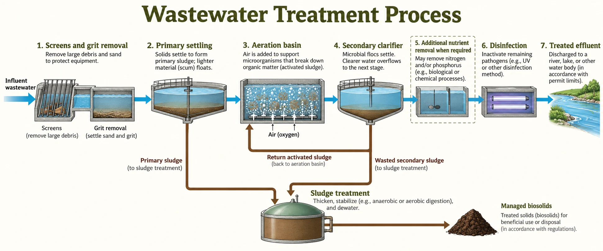
Sewage treatment removes solids, biodegradable material and other contaminants before discharge or reuse. Physical separation, biological treatment, nutrient removal and disinfection serve different purposes. A sanitation-access statistic is not identical to the proportion of wastewater safely treated.
Primary Treatment
- Processes: Physical removal; screens (remove large solids), grit chambers (sand/gravel settles), settling tanks (suspended solids settle by gravity)
- Performance: Primary settling removes much of the settleable solids and some associated oxygen-demanding material. Removal depends on influent and operation; dissolved nutrients and pathogens generally require further controls.
- Residuals: Screens and grit produce separate wastes, while primary settling produces sludge and surface scum. Sludge enters a solids-treatment pathway; it is not simply returned to the main secondary water-treatment flow untreated.
- Limitations: Does not remove dissolved pollutants; pathogens remain; dissolved organics, nutrients not removed; effluent still polluted, needs secondary
- Role: Preliminary and primary stages protect equipment and reduce loads on later processes. The treatment train must match discharge or reuse requirements; primary treatment alone cannot be assumed sufficient for every receiving water.
Secondary Treatment
- Activated sludge: Aerated microorganisms consume biodegradable organic material, converting it into biomass, and other products. BOD is a measure of oxygen demand, not a substance that microbes eat.
- Process: Aeration provides ; promotes rapid bacterial growth; microorganism flocs settle in secondary clarifiers; sludge recycled (some wasted); effluent extracted
- Performance: Proper secondary treatment achieves substantial BOD and suspended-solids removal. Nitrification converts ammonia to nitrate but does not by itself remove total nitrogen; denitrification or other pathways are needed. Pathogen reductions vary and do not replace disinfection.
- Alternatives: Trickling filters (fixed-film bioreactors), lagoons (natural aeration/sunlight), rotating contactors, membrane bioreactors (high efficiency, expensive)
- Sludge: Primary solids and excess biological sludge need thickening, stabilization and appropriate dewatering and management. Quantity depends on loading and process; specify dry solids versus wet sludge before comparing masses.
- Energy: Aeration is often a major electricity demand. Efficient blowers, diffusers, process control and appropriate oxygen targets can save energy, but cost and energy shares vary among plants.
- Cost vs. Benefit: Moderate cost; good removal efficiency; residual pollutants (nitrogen/phosphorus, trace organics, some pathogens) require tertiary treatment for reuse
Tertiary and Advanced Treatment
- Advanced separation: Media filtration removes particles; microfiltration and ultrafiltration remove selected particle and microbe sizes, while reverse osmosis also rejects many dissolved substances. Membranes are not interchangeable and create residual streams requiring management.
- Nutrients: Nitrogen removal often combines aerobic nitrification with anoxic denitrification. Phosphorus may be removed by chemical precipitation or enhanced biological processes. Performance and cost depend on the treatment targets and design.
- Oxidation: Ozone and advanced oxidation can transform some organic contaminants and inactivate organisms. UV disinfection and UV-based advanced oxidation are different applications; transformation products, dose and water quality matter.
- Activated Carbon: Adsorbs dissolved organics; removes trace pollutants (pharmaceuticals, pesticides); saturation requires regeneration/replacement
- Reuse: Suitability is use-specific. Irrigation, industrial use, recharge and potable reuse require different treatment, monitoring and barriers; a “tertiary” label alone does not establish drinking-water quality.
- Costs: Advanced treatment adds capital, energy, chemicals, maintenance and residual-management needs. Costs depend on scale and targets; benefits can include water supply reliability and protection of sensitive ecosystems.
- Trace contaminants: Conventional plants remove some pharmaceuticals, particles and other emerging contaminants to varying degrees. Additional barriers may be needed; a lower effluent concentration can also reflect transfer into sludge rather than destruction.
Disinfection
- Chlorination: Chlorine can inactivate many pathogens when concentration and contact time are adequate. Organic matter and chemistry influence disinfection by-products. Wastewater may require dechlorination before discharge to protect aquatic life.
- UV: Appropriate UV dose damages microbial genetic material and can effectively inactivate Cryptosporidium. Turbidity and shielding affect performance. UV leaves no protective disinfectant residual, and system operation and validation are essential.
- Ozone: A strong oxidant that can inactivate organisms and transform some organics. It leaves no lasting disinfectant residual and can form by-products, including bromate where bromide is present.
- Validation: Required pathogen reductions depend on organism and intended use, often expressed as log reductions. A generic 99.9% figure is not guaranteed by any disinfectant name; concentration, contact or dose, and water quality control performance.
- Trade-offs: Chlorine, UV and ozone differ in cost, residual protection, by-products and organism sensitivity. Multiple barriers and monitoring are selected for the specific treatment and distribution system.
- Implementation: Reliable supply, operator training, power, maintenance and testing sustain disinfection. A technically suitable process may fail if these operating requirements are not met, regardless of national income category.
Global Coverage and Challenges
- Coverage: Sewered treatment, on-site sanitation and safely managed services are different indicators. WHO/UNICEF’s 2025 report estimates 2.1 billion people lacked safely managed drinking water in 2024; do not describe that number as people lacking sewage treatment.
- Variation: Treatment access and performance differ among and within countries, including between urban, rural and informal settlements. Connection to a sewer does not guarantee that wastewater receives adequate treatment.
- Investment: Collection, treatment, on-site systems and ongoing operation all require funding. Global cost estimates depend on service targets, baseline year and scope; financing construction alone does not ensure sustained service.
- Loading:. Use consistent flow and concentration units to obtain pollutant mass per time. Population-based design also requires an appropriate per-capita flow and assumptions about industrial inputs or infiltration.
- Design flow: Domestic use, industrial inputs, infiltration and stormwater connections influence influent. Average flow, peak flow and pollutant loading are separate design quantities; a universal per-capita volume or peak multiplier is unreliable.
- Maintenance Requirements: Skilled operators needed; equipment maintenance; chemical supply; monitoring; often lacking in resource-limited settings
- SDG 6: The 2030 goals include safe drinking water, sanitation and improved wastewater management. Progress indicators assess different services and targets; “60% on track” is not a single measure of the whole goal.
Exam tip: Trace water and solids separately: screening and settling, biological conversion, secondary clarification, additional treatment and disinfection. Identify the return-sludge loop and wasted solids. Explain BOD, nitrogen transformation versus removal, and why clear-looking effluent is not automatically pathogen-free or potable.
Worked example: BOD load and removal
Assume an average flow of 200,000 L per day through a hypothetical plant, with matching influent and effluent periods and negligible flow change. Influent is 180 and effluent is 18 .
The outlet load is 3.6 kg per day, leaving 32.4 kg per day removed from the measured BOD load. When flows differ, calculate inlet and outlet mass loads rather than compare concentrations alone. Treatment can convert organics or transfer material to sludge, so removal is not necessarily destruction of every constituent.
8.12 Lethal Dose 50% ()
Definition and Methodology
is the estimated dose producing death in half a defined test population under specified conditions. Report species, route, formulation and observation period, usually with dose normalized to body mass. It measures acute lethal potency, not a daily safe intake.
Test Specificity and Variability
- Species: Absorption, metabolism, target sensitivity and elimination differ among species. Animal results inform assessment but cannot be scaled to humans using body mass alone; uncertainty must be evaluated.
- Route: Oral and dermal values can differ. Inhalation tests commonly report , an airborne concentration over a specified exposure time, rather than an administered dose per body mass.
- Test population: Age, sex, strain and health affect response. A result describes the tested population and protocol; sensitivity in other populations requires additional evidence.
- Environmental Factors: Temperature, food, water availability, stress affect response; controlled lab conditions may not reflect real-world exposure
- Statistics: is estimated from a dose–mortality relationship with sampling uncertainty. Responses need not follow a normal distribution, and the median lethal dose is not a boundary below which no deaths or other effects occur.
- Comparison: If hypothetical chemicals A and B have oral values of 20 and 200 in the same test system, A has greater acute lethal potency on that basis. This does not rank chronic, ecological or real-world exposure risks.
Toxicity Classification
- Classification context: Acute-toxicity categories depend on the adopted system and exposure route. The following oral acute-toxicity-estimate cutoffs illustrate OSHA’s four-category system; they are not the older “extreme to nontoxic” scale.
- Oral category 1: An acute toxicity estimate at or below 5 . The category is route-specific and does not specify a lethal amount for a particular person.
- Oral category 2: Above 5 and at or below 50 . Compare test conditions and formulation before assigning or comparing categories.
- Oral category 3: Above 50 and at or below 300 . Acute lethal potency remains separate from exposure likelihood and chronic effects.
- Oral category 4: Above 300 and at or below 2,000 . A larger estimate does not imply that a substance is safe to ingest or lacks other hazards.
- Beyond these categories: OSHA does not adopt GHS acute-toxicity category 5. Falling outside categories 1–4 is not a general “nontoxic” classification; other hazard classes and endpoints still matter.
- Water example: Excessive water intake can cause dangerous electrolyte imbalance. Even essential substances can harm under particular exposure conditions; the absence of a routine value does not prove unlimited safety.
- Interpretation: Lower comparable values indicate greater acute lethal potency. Actual risk also depends on dose, route, duration, exposure probability and population; handling decisions require the substance’s complete safety information.
Limitations of Approach
- Acute endpoint: Lethal-dose tests assess mortality following a specified acute exposure and observation period. They do not adequately describe chronic disease, developmental injury or other sublethal effects.
- Missing Sublethal Effects: Reproductive toxicity, developmental effects, immune suppression, behavioral changes not captured; functional impairment occurs before death
- Extrapolation: Pharmacokinetic and biological differences affect animal-to-human inference. There is no fixed hundred-fold difference in metabolism between all rodents and humans.
- Susceptibility: A test population cannot represent every human life stage or health condition. Additional studies, modeling and appropriate uncertainty factors inform assessment; factors should not double-count the same uncertainty.
- No safety threshold: identifies a median lethal dose, not a no-effect threshold. Effects can occur below it, and lower-dose chronic or endocrine endpoints require their own dose–response evidence.
- Other measures: NOAEL is the highest tested dose without a detected adverse effect for the endpoint; LOAEL is the lowest tested dose with one. describes a defined median effective dose or half-maximal graded response, depending on context; benchmark-dose methods use modeled data.
- Broader assessment: Modern testing uses multiple endpoints, exposure information and alternatives that reduce animal use where appropriate. Acute toxicity remains one component; it is not replaced by a single universal substitute measure.
Reference Dose Derivation
- Reference dose: An RfD is derived from an appropriate noncancer point of departure, such as a chronic-study NOAEL or benchmark-dose lower bound, with uncertainty adjustments. A NOAEL cannot be inferred by taking a fixed fraction of .
- Simplified derivation:. The point of departure and combined factors must be justified for the chemical, endpoint, database and exposure duration.
- Factors: Separate adjustments may address animal-to-human extrapolation, human variability, study duration, database gaps or use of a LOAEL. Defaults are often three or ten, but the combination is evidence-based rather than a mandatory fixed total.
- Hypothetical example: A suitable NOAEL of 1 divided by a combined uncertainty factor of 100 gives an RfD of 0.01 . This is a noncancer assessment estimate, not proof of zero risk or a value derived from an acute .
- Water screening:. Body mass multiplies an intake per body mass, while water consumption is in the denominator. Allocation accounts for other exposure sources. This simplified screen is not itself an enforceable drinking-water standard.
- Uncertainty: Study quality, endpoint choice, model fit and exposure assumptions affect the result. Uncertainty factors support protective estimates; they neither erase all uncertainty nor justify ignoring low-dose or sensitive-life-stage evidence.
Exam tip: Read as a test-specific median lethal dose and distinguish it from and chronic endpoints. Use comparable tests to rank acute potency. Derive an RfD from a justified point of departure, not an arbitrary fraction of , and check units in exposure calculations.
Worked example: a reference-dose screening calculation
For a fictional chemical, suppose an appropriate noncancer study supports a point of departure of 1 and a combined uncertainty factor of 100.
For a hypothetical water-only screen, take body mass BW of 60 kg, an allocation fraction RSC of 0.20 and water intake IR of 2 L per day.
This is a classroom calculation, not a limit for a real chemical, legal standard or individual recommendation. Actual assessments require a validated reference value, chemical-specific exposure information and the applicable regulatory framework.
8.13 Dose Response Curve
Fundamental Principles
Dose–response describes how a defined biological endpoint changes with exposure. The relationship may be monotonic or nonmonotonic and varies with route, duration and organism. Distinguish the fraction of a population responding from the magnitude of a response in one organism.
Classical Sigmoid (S-Shaped) Curve
- Three Regions:
- Lower-dose region: A study may detect no adverse response at its lower tested doses. Detection limits, sample size and endpoint choice matter; absence of a detected effect is not proof of a universal zero-risk threshold.
- Rising region: The measured response increases over a dose interval. Slope describes the rate of change for the chosen axes; the dose needed for a specified response describes potency. These are related but distinct features.
- Plateau: A graded response may approach a biological maximum; a quantal mortality curve approaches all tested individuals responding. Receptor saturation is one mechanism, not the explanation for every plateau.
- Curve shape: Receptor dynamics can produce an S-shaped graded response, while differences in individual thresholds can produce an S-shaped population curve. Axis scaling also changes appearance; identify the endpoint and axes first.
- : Depending on the definition, the dose giving a specified effect in 50% of a population or half of a maximum graded effect. It is not automatically an inflection point for every fitted model or evidence of “moderate safety.”
- : A median dose for the specific quantal endpoint of death. A mortality curve describes proportions dying, while other adverse effects may occur at doses below those producing substantial mortality.
- Transformations: Plotting dose on a logarithmic axis can spread low doses but does not itself make a sigmoid straight. A logit transformation of response probability can be linear in log-dose for a specified logistic model; this is a modeling assumption to assess against data.
Critical Curve Components
- NOAEL: Highest tested dose at which the study detects no adverse effect for the evaluated endpoint. It depends on dose spacing and statistical power and is not a precisely measured boundary between safe and unsafe exposure.
- LOAEL: Lowest tested dose with a detected adverse effect. It is study- and endpoint-specific; the true biological onset cannot be located exactly merely from this tested value.
- Potency: Lower comparable values indicate greater potency for the same defined effect and test conditions. This does not establish the greatest possible effect, chronic hazard or real-world risk.
- Margin of exposure:. Compare compatible units and exposure durations. The adequacy of a margin depends on the point of departure and uncertainties; a margin above 100 is not a universal safety certificate.
- Slope: A steep curve means the response changes over a narrower dose range on the stated axes. A curve can be shifted left or right without changing slope; potency and slope should not be equated.
- Threshold interpretation: Some endpoints are assessed with threshold models and others with different approaches. A study’s NOAEL does not establish a threshold for every endpoint, duration or person.
- Reference value: A suitable point of departure and uncertainty adjustments support an RfD for noncancer effects. It is an assessment estimate for specified exposure conditions rather than a daily dose guaranteed harmless to everyone.
Nonmonotonic responses and hormesis
- Nonmonotonicity: The slope changes sign within the measured dose range, for example in U-shaped or inverted-U patterns. A low-dose effect and a nonmonotonic curve are not synonyms.
- Hormesis: A biphasic response involving stimulation at lower doses and inhibition or harm at higher doses for a particular endpoint. Whether a measured change benefits the whole organism requires evidence; not every nonmonotonic response is hormesis.
- Endocrine examples: Some hormone or BPA experiments show endpoint-specific nonmonotonic patterns. Evaluate species, timing, dose range, controls and replication; one pair of atrazine concentrations does not establish a universal rule.
- Hormone signaling: Different receptors, feedback and downstream pathways can respond at different concentrations. Physiological signaling and toxicity are distinct endpoints, so curves must state precisely what was measured.
- Mechanisms: Multiple receptor types with different sensitivities; feedback loops; adaptive responses; redundant pathways; complex biology
- Testing challenge: Suitable dose spacing, sensitive endpoints, developmental timing and replication are needed to characterize complex curves. High-dose testing alone may not predict lower-dose responses for a nonmonotonic relationship.
- Prevalence: Whether nonmonotonicity is detected depends on the tested chemical, endpoint and design. An unqualified percentage of all chemicals is not established by one set of experiments.
- Evaluation: Assess data quality, effect size, reproducibility and biological mechanism. A proposed hormetic effect does not by itself justify exposure or overturn protective guidance.
Population Variability and Regulatory Application
- Population variation: Genetics, age, health and prior exposure influence responses. A quantal curve summarizes a distribution; neither a fixed ten-fold range nor a particular statistical distribution fits every population.
- Vulnerable Subpopulations: Children (immature systems, higher metabolism), pregnant women (fetal effects, altered pharmacokinetics), elderly (declining kidney/liver function), diseased (multiple medications, comorbidities)
- Genetics: Variants in metabolic enzymes and other pathways can affect internal dose and susceptibility. Faster metabolism may detoxify a substance or activate a toxic metabolite; the direction depends on the chemical.
- Uncertainty adjustments: Factors address identified limitations, including interspecies extrapolation and human variability. Avoid automatically multiplying an extra “sensitive people” factor that duplicates variability already considered.
- Water values: Intake-based screening multiplies an appropriate reference dose by body mass and an allocation fraction, then divides by daily water intake. National standards also reflect legal, analytical and treatment considerations.
- Exposure Variability: Real-world exposure variable; some people higher intake (occupation, diet, behavior); models use average + upper percentile scenarios
- Mixtures: Dose addition or response addition may be suitable under different assumptions; synergistic and antagonistic interactions are also possible. Mixture assessment must state the shared mechanism or endpoint rather than simply sum all observed responses.
Exam tip: Identify axes, endpoint, exposure period and population. Separate potency from slope and graded response from incidence. Interpret NOAEL and LOAEL as tested levels, and distinguish nonmonotonicity from hormesis. Support risk conclusions with exposure as well as hazard evidence.
Practice: read a hypothetical mortality dataset
| Dose | Mortality observed |
|---|---|
| 1 | 0% |
| 5 | 20% |
| 10 | 50% |
| 20 | 80% |
| 50 | 100% |
The observed median lethal dose is near 10 for this hypothetical experiment. A fitted estimate would also use sample counts and uncertainty. Zero observed mortality at 1 does not establish a chronic NOAEL or prove absence of reproductive, neurological or other sublethal effects.
In a logistic model with probability p and positive dose D, a logit can be modeled as linear in log-dose:
The reference dose Dref makes the logarithm’s argument dimensionless. This equation is one statistical model; plotting dose on a logarithmic axis alone does not transform response probability into a straight line.
8.14 Pollution and Human Health
Global Health Burden
Health burden: A 2022 Lancet Planetary Health update estimated approximately nine million premature deaths attributable to pollution in 2019. This is a model-based estimate for a defined year and set of risks, not a current annual census or a sum to combine with overlapping risk categories.
Pollution-Related Deaths Breakdown
- Air: Particle and other air-pollutant exposures contribute to cardiovascular and respiratory disease and cancer. Ambient and household estimates can overlap, so their attributable death counts require joint-risk methods rather than simple addition.
- Unsafe WASH:WHO estimated that adequate drinking water, sanitation and hygiene could have prevented at least 1.4 million deaths in 2019. This includes multiple health pathways and is broader than directly drinking polluted water.
- Lead: Exposure can damage neurodevelopment and contribute to cardiovascular and other disease. Burden estimates depend on data and model assumptions; preventing exposure remains important even where overt poisoning is not diagnosed.
- Asbestos: Inhaled fibers can cause mesothelioma, lung cancer and asbestosis, often after long latency. Occupational and environmental exposure histories matter; a fixed latency or undated global death total does not describe every case.
- Pesticides: Acute poisoning can follow occupational, accidental or intentional exposure. Chronic effects and acute events are measured differently, and reporting gaps affect estimates. Training, exposure controls, safer practices and health services address different risks.
- Other exposures: Mercury, radon, tobacco smoke and polluting household fuels cause distinct health concerns. Some are already included within broader air-pollution estimates, making careful definitions essential to avoid double-counting.
- Uncertainty: Incomplete exposure data and limited knowledge of mixtures complicate attribution. Estimates include uncertainty ranges and assumptions; gaps can cause underestimation, but not every uncertainty necessarily shifts a result in the same direction.
Vulnerable Populations
- Children: Developmental sensitivity, hand-to-mouth behavior and exposure relative to body mass can increase vulnerability. Lead and methylmercury can affect neurodevelopment; one fixed IQ loss per blood-lead increment does not apply to every child or exposure range.
- Pregnancy: Some pollutants cross the placenta or affect maternal physiology, creating sensitive developmental windows. Outcomes depend on chemical, dose and timing; exposure does not guarantee a permanent fetal effect.
- Elderly: Comorbidities (existing cardiovascular/respiratory disease); compromised kidney/liver function; medication interactions; higher pollution sensitivity
- Poor/Low-Income: Greater exposure (live near factories, highways, dumps); inadequate healthcare; malnutrition reduces immune function; limited access to clean water/food; double burden (exposure + less resilience)
- Workers: Agriculture, construction and mining can involve pesticides, dust, fibers or metals. Substitution, engineering controls, work practices and suitable protection reduce exposure; actual protection depends on implementation and enforcement.
- Indigenous/Arctic Populations: Bioaccumulation in traditional foods; exposure despite no production responsibility; environmental justice issue
- Disparities: Historical discrimination, land use, housing and investment can concentrate exposure in some racial or ethnic communities. Measure the specific location and pollutant rather than assume a uniform pattern for every group.
Environmental Justice
- Unequal burden: Exposure and susceptibility can differ by income, race, occupation and place. Compare monitored or modeled concentrations, access to services and health outcomes; a universal two- or three-fold multiplier conceals local variation.
- Historical processes: US redlining and other discriminatory policies shaped investment and housing opportunities. These legacies can interact with transport and industrial land use to affect present exposure; pathways differ among neighborhoods.
- International burdens: Pollution-intensive production and waste trade can shift exposure across borders. Supply chains, domestic activity, regulation and consumption all matter; responsibility cannot be reduced to a simple north–south split.
- Participation: Communities may face barriers to information, decision-making and enforcement. Meaningful participation, accessible monitoring and accountable institutions can improve protection and the distribution of benefits.
- Costs: Medical expenses, lost income, caregiving and reduced productivity can disproportionately burden households with fewer resources. National or global valuations require a defined year, method and set of outcomes.
- Community action: Environmental-justice efforts seek equitable protection and meaningful involvement. Cases such as Flint highlight infrastructure, exposure, accountability and public trust; their legal conclusions are case-specific.
Disease Burden and DALYs
- DALYs (disability-adjusted life years) measure healthy life lost through premature mortality and disability. They allow comparisons using compatible methods, but are neither a death count nor a direct measure of financial costs.
- DALY comparisons: Use the same study year, geography and method when comparing burdens. Unsafe water can be part of a pollution assessment, so comparing or adding overlapping categories as if independent creates errors.
- Chronic effects: Long-term exposures contribute to different diseases through pollutant-specific pathways. Latency varies by outcome and dose; causal assessment combines epidemiology, toxicology and exposure evidence.
- Combined pressures: Pollution, nutrition, housing, access to care and existing disease can interact. “Synergy” specifically means an effect beyond a stated additive expectation and should not be assumed for every combination.
- Economic assessment: Healthcare, lost production and welfare losses are different valuation components. State the boundary and avoid treating a historical estimate as current expenditure or a universally comparable GDP share.
- Prevention: Many exposure-control measures provide health and economic benefits. Cost per DALY avoided depends on intervention and context; no single cost ratio proves every prevention option cheaper than every treatment.
Exam tip: Connect source, exposure, dose, susceptibility and effect. Define attributable deaths and DALYs, identify dates and overlapping risks, and explain environmental justice using specific exposure and participation pathways. Distinguish a modeled population burden from an individual diagnosis.
DALYs: keep the components distinct
Disability-adjusted life years combine years of life lost due to premature death with years lived with disability, using the chosen study’s disability weights and methods.
A DALY is one year of healthy life lost. It is not a death count or a healthcare bill. Compare estimates from compatible methods and avoid adding overlapping health-risk categories.
8.15 Pathogens and Infectious Diseases
Waterborne Diseases and Global Burden
Water-related infectious disease includes fecal–oral transmission through contaminated water or food and other environmental pathways. Unsafe sanitation and hygiene amplify exposure. Disease-specific and WASH-attributable death estimates use different definitions and should not be treated as one interchangeable total.
Major Waterborne Pathogens
- Cholera: Toxigenic Vibrio cholerae can cause severe watery diarrhea and rapid dehydration, although many infections are mild or asymptomatic. Safe water, sanitation, hygiene and vaccination support prevention; suspected severe illness requires prompt medical care.
- Typhoid:Salmonella Typhi spreads through fecally contaminated food or water and can cause prolonged fever and systemic illness. Some people become long-term carriers. Vaccination, sanitation and appropriate clinical treatment address different parts of control.
- Dysentery: Bloody diarrhea can result from organisms such as Shigella or Entamoeba histolytica; the latter is a protozoan. Different causes require different assessment, so dysentery is not one bacterial species or one fixed fatality rate.
- Rotavirus: A major cause of gastroenteritis in young children, with dehydration risk. Vaccination has reduced severe disease where implemented; local burden depends on vaccination coverage, care access and other pathogens.
- Hepatitis A: A fecal–oral viral infection affecting the liver. Unlike hepatitis B and C, hepatitis A does not cause chronic infection, although acute illness can be severe. Vaccination, hygiene and safe food and water reduce transmission.
- Cryptosporidium: A protozoan parasite causing diarrhea, potentially severe in immunocompromised people. Its oocysts tolerate routine chlorination; effective filtration and validated UV or other appropriate treatment provide additional barriers.
- Giardia: A protozoan parasite transmitted through ingestion of cysts, including contaminated water or person-to-person pathways. Appropriate filtration and validated disinfection methods reduce waterborne transmission; clinical treatment is a separate measure.
- Helminths: Transmission differs among worms. Schistosome larvae penetrate skin during contact with contaminated freshwater; hookworm often enters through contaminated soil, while roundworm eggs are ingested. Sanitation, suitable exposure prevention and disease-specific control are needed, not water treatment alone.
Transmission and Risk Factors
- Fecal-Oral Route: Contaminated water/food ingested; direct contact with sewage; pathogens survive water transit; poor sanitation amplifies risk
- Water Contamination Sources: Untreated sewage discharge, animal waste (livestock, wildlife), leaking septic systems, flooding during heavy rain, inadequate treatment
- Access: WHO/UNICEF’s 2025 report estimates 2.1 billion people lacked safely managed drinking water in 2024. This indicator combines source quality, availability and access; it does not mean that all these people have no water source, nor that 80% of all disease is waterborne.
- Food Contamination: Produce/seafood grown in/from contaminated water; shellfish bioaccumulate pathogens; meat/dairy processing water source
- Seasonality: Floods can spread fecal material and disrupt treatment, while drought can reduce safe supplies or concentrate some contaminants. Pathogen ecology and infrastructure determine local patterns; outcomes are not identical in every monsoon or drought.
- Socioeconomic Risk: Poverty → inadequate sanitation → disease; cycle difficult to break; requires infrastructure investment
Vulnerable Populations
- Young children: Diarrheal disease remains a major cause of childhood death, with malnutrition and impaired immunity increasing risk. Dehydration can develop rapidly; safe WASH, vaccination and access to appropriate care are complementary protections.
- Immunocompromised people: Some infections, including cryptosporidiosis, can be more severe or persistent. Immune status and access to effective treatment affect outcomes; one laboratory cutoff does not describe every person’s risk.
- Malnourished: Inadequate nutrition → poor immune function; disease severity increased; higher mortality rate; vicious cycle (disease prevents nutrient absorption)
- Underserved communities: Limited reliable water, sanitation and healthcare can increase exposure and delay care. Infrastructure, affordable services and community participation improve protection; individual behavior alone cannot compensate for every service gap.
- Migrants/Displaced: Refugee camps, slums lack sanitation; crowding increases transmission; outbreak risk high; humanitarian crisis component
Climate Change and Emerging Diseases
- Climate Impacts on Waterborne Disease: Flooding increases pathogen spread; drought concentrates pathogens; temperature changes alter pathogen seasonality/survival; precipitation pattern shifts affect water availability
- Vector-borne disease: Temperature and rainfall can alter mosquito survival, development and distribution. Malaria, dengue and Zika are transmitted by vectors rather than by drinking water; housing, vector control, travel and immunity also shape transmission.
- Malaria: WHO estimates 282 million cases and 610,000 deaths worldwide in 2024. Mosquito ecology, parasite biology and health services influence risk. Climate change can alter suitable conditions, but does not guarantee uniform poleward expansion everywhere.
- Dengue: A mosquito-borne viral disease affected by urban conditions, travel, vector ecology and climate. Vaccines exist with specific eligibility and program recommendations; vaccination does not replace mosquito control and other prevention.
- Cholera and climate: Environmental conditions can affect Vibrio ecology, while disruption of water and sanitation strongly influences outbreaks. Climate is one factor among infrastructure, movement, immunity and public-health response.
- Zoonoses: Land-use change, wildlife contact, livestock systems and trade can alter opportunities for pathogens to cross species. Transmission and emergence are pathogen-specific; a broad spillover framework does not establish the exact origin of every outbreak.
Prevention and Treatment
- Prevention: Reliable safe water, effective sanitation and hygiene interrupt multiple transmission pathways. Combine infrastructure, safe storage, maintenance, monitoring and education; no universal fraction of all infectious disease is prevented by one measure.
- Water barriers: Validated boiling, filtration and disinfection methods target different hazards. Turbidity, organism resistance, contact time and recontamination affect performance. Removing microbes does not necessarily remove dissolved chemicals, and generic sunlight exposure is not a guaranteed treatment protocol.
- Vaccines: Vaccines are available for several diseases, including rotavirus, cholera, typhoid and hepatitis A. Eligibility, schedules, effectiveness and availability differ; disease prevention still requires safe WASH and appropriate local programs.
- Care: Oral rehydration solutions replace water and electrolytes lost during diarrhea, while severe illness may need additional medical care. Antibiotics are used selectively for appropriate infections, not all diarrhea; prevention and clinical treatment answer different needs.
- Economics: WASH investment can provide substantial health and social benefits, but costs depend on geography, service level, reliability and maintenance. Compare like-for-like costs and outcomes rather than one universal per-person price.
- SDG 6: The 2030 agenda includes universal drinking-water and sanitation access and improved water quality. Progress depends on investment, sustainable operation, governance and inclusion; targets are goals rather than a guarantee that every country is on track.
Exam tip: Match each pathogen to its transmission route and the barriers that interrupt it. Distinguish waterborne, soil-transmitted and mosquito-borne disease. Explain how treatment resistance, sanitation, maintenance, poverty and climate interact, and distinguish disease burden from access-to-service indicators.
Unit 8 revision checklist: all 15 topics
All 15 Topics
- 8.1 Sources (point vs. nonpoint)
- 8.2 Human impacts (habitat, invasives)
- 8.3 Endocrine disruptors
- 8.4 Wetlands & mangroves
- 8.5 Eutrophication
- 8.6 Thermal pollution
- 8.7 POPs
- 8.8 Bioaccumulation/magnification
- 8.9 Solid waste
- 8.10 Waste reduction
- 8.11 Sewage treatment
- 8.12
- 8.13 Dose-response
- 8.14 Human health
- 8.15 Pathogens
Key Points
- Point = traceable; nonpoint = diffuse
- Habitat loss and degradation are major biodiversity pressures, interacting with other threats.
- Invasive species can cause major harm; their relative importance differs among ecosystems.
- POP accumulation depends on chemical properties, uptake, elimination and tissue basis.
- Hypoxic zones vary in area, duration and severity; counts require a dated inventory.
- Population health-burden estimates need a study year, risk definition and uncertainty.
- Wetland-loss estimates depend on baseline and definition; the 2025 outlook reports major loss since 1970.
- Unsafe WASH contributes to multiple diseases; waterborne and vector-borne routes differ.
- Curve shape depends on endpoint, population and axes; not every response is sigmoid.
- Environmental justice examines unequal exposure, susceptibility, participation and protection.
- measures test-specific acute lethal potency and is not a daily safe intake.
- BMF compares matched predator and prey concentrations; no fixed trophic multiplier applies.
- Bioaccumulation reflects uptake and removal over time, including possible depuration.
- Nutrient enrichment can increase production and oxygen demand, especially where replenishment is limited.
- Nonmonotonicity means a change in slope direction; it is not synonymous with hormesis.
AP Exam Strategy for Unit 8
For each topic, explain a source, transport or exposure pathway, mechanism, effect and suitable control. Trace eutrophication through respiration and oxygen replenishment, and distinguish it from algal toxicity. Compare BAF and BMF using explicit units and matched tissue bases. Follow both water and sludge through treatment, and assess containment and residuals in waste disposal. Interpret toxicity curves using defined axes and endpoints; distinguish lethal-dose measures from noncancer reference doses. Use dated, nonoverlapping statistics and explain how social conditions influence exposure and protection. Practise loads, dilution, removal efficiency, half-life, thermal response and exposure calculations, always showing units and assumptions.
APES Unit 8 study notes FAQs
What do APES Unit 8 study notes cover?
These Aquatic and Terrestrial Pollution notes cover all 15 topics, including water pollution, endocrine disruptors, wetlands, eutrophication, persistent pollutants, bioaccumulation, solid waste, sewage treatment, toxicology and environmental health. Detailed explanations, diagrams and worked calculations support revision.
How do bioaccumulation and biomagnification differ?
Bioaccumulation is the buildup of a substance within an organism when uptake exceeds elimination over time. Biomagnification is an increase in comparable tissue concentrations across trophic levels. Whether either occurs depends on chemical properties, exposure and the food web.
Why can eutrophication lower dissolved oxygen?
Excess nutrients can stimulate aquatic production. Respiration and microbial decomposition of organic matter consume oxygen, while stratification may limit replenishment. Severe oxygen depletion can harm aquatic organisms. Nutrient enrichment and toxin production are distinct processes.
What happens in primary and secondary sewage treatment?
Primary treatment physically separates settleable solids and floating material. Secondary biological treatment reduces biodegradable organic matter, followed by biomass separation. Nutrient removal and disinfection address additional goals; effectiveness varies by treatment design and operation.
Does a median lethal dose establish a safe chronic exposure?
No. A median lethal dose describes mortality under a defined experimental protocol. It does not establish a chronic no-adverse-effect level or a safe daily intake. Chronic risk assessment requires appropriate endpoints, exposure information, a supported point of departure and justified uncertainty factors.
How much of the APES multiple-choice section is Unit 8?
College Board assigns Aquatic and Terrestrial Pollution a 7–10% weighting in the multiple-choice section. Practise pollutant pathways and controls, interpret dose-response and environmental data, and calculate loads, removal percentages and accumulation factors using consistent units.