
Unofficial study guide
Early Solutions to the 2026 AP Microeconomics FRQs | Step by Step
Complete solutions for the user-provided 2026 paper, including game theory, monopoly, competitive-firm costs, free trade, tariffs, every calculation, and every required graph label.
How to Use This Solution
- Read each reasoning section to understand the economic logic.
- Use each green final-answer box as a model for a concise AP-style response.
- On every calculation question, show the formula, substitute the numbers, and state the units.
- On every graph, label both axes, all required curves, the requested prices and quantities, and any shaded area.
At-a-Glance Answer Key
| Part | Answer |
|---|---|
| 1A | Rail. Feram earns $50 million instead of $40 million when Ocel chooses Sheets. |
| 1B | Ocel has no dominant strategy: Beams is better against Truck, but Sheets is better against Rail. |
| 1C | Unique Nash equilibrium: (Rail, Sheets), with payoffs $50 million and $75 million. |
| 1D | Subtract $20 million from each Feram payoff in the Rail row: (30,75) and (10,25). |
| 1E | Monopoly output is where MR = MC; price is read from demand; ATC lies below price at that quantity; deadweight loss lies between demand and MC from monopoly output to the efficient output. |
| 1F | Price remains the same. A lump-sum tax raises fixed cost and ATC, but not MC. |
| 2A | Perfect competition. |
| 2B | AVC at 4 helmets is $30 per helmet. |
| 2C | Economic profit at 5 helmets is $65. |
| 2D | Profit-maximizing quantity is 8 helmets. |
| 2E | Market price decreases as entry shifts market supply right. |
| 3B(ii) | Total economic surplus increases under free trade. |
| 3C(ii) | Domestic producer surplus increases after the tariff. |
Duopoly Game, Merger, Monopoly, and Tax
The original payoff matrix reports profits in millions of dollars. The first number in each cell is Feram's profit; the second is Ocel's profit.
| Feram | Ocel | |
|---|---|---|
| Sheets | Beams | |
| Truck | (40,95) | (20,125) |
| Rail | (50,75) | (30,25) |
Part A: Feram's Best Response When Ocel Chooses Sheets
Part B: Does Ocel Have a Dominant Strategy?
A dominant strategy must be Ocel's best choice regardless of Feram's action.
| Feram's action | Ocel: Sheets | Ocel: Beams | Ocel's best response |
|---|---|---|---|
| Truck | 95 | 125 | Beams, because \(125>95\) |
| Rail | 75 | 25 | Sheets, because \(75>25\) |
Part C: Nash Equilibrium
- If Ocel chooses Sheets: Rail gives Feram 50 instead of 40.
- If Ocel chooses Beams: Rail gives Feram 30 instead of 20.
Thus, Rail is Feram's strictly dominant strategy. Given that Feram chooses Rail, Ocel compares 75 from Sheets with 25 from Beams, so Ocel chooses Sheets. The cell (Rail, Sheets) is therefore the only cell containing mutual best responses.
Part D: A $20 Million Increase in Feram's Rail Cost
| Feram | Ocel | |
|---|---|---|
| Sheets | Beams | |
| Truck | (40,95) | (20,125) |
| Rail | (30,75) | (10,25) |
Only the first number in each Rail cell changes.
Part E: Acier as a Monopoly
After the merger, Acier is the only steel producer, so it faces the market demand curve.
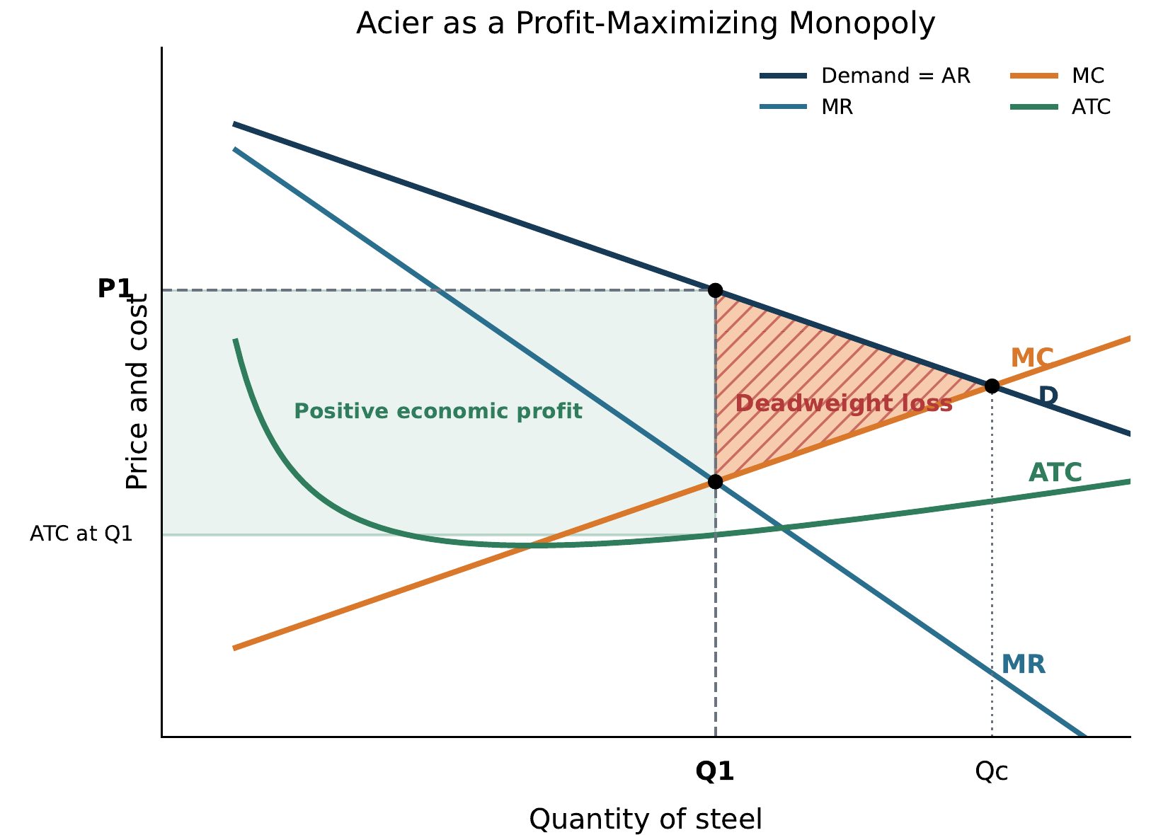
- Draw a downward-sloping demand curve labeled D or D = AR. Draw the marginal-revenue curve below demand.
- Draw marginal cost, MC. The profit-maximizing quantity is where MR = MC; label it \(Q_1\).
- Move vertically from \(Q_1\) to the demand curve. The corresponding price is the monopoly price \(P_1\).
- Draw ATC so that ATC at \(Q_1\) is below \(P_1\). This is consistent with positive economic profit: \(\pi=[P_1-ATC(Q_1)]Q_1>0\).
- The allocatively efficient quantity is where demand equals marginal cost, labeled \(Q_c\). Since a monopolist restricts output, \(Q_1<Q_c\).
- Completely shade the area between demand and marginal cost from \(Q_1\) to \(Q_c\). That triangle is deadweight loss because those mutually beneficial units are not produced.
Part F: Effect of a Lump-Sum Tax on Acier's Price
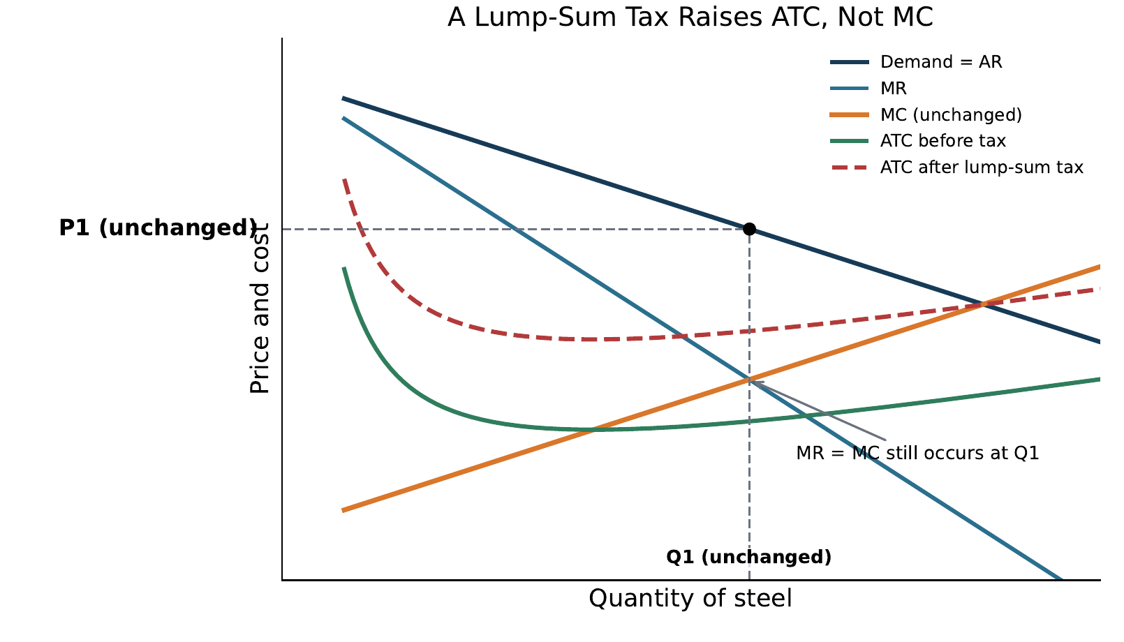
- A lump-sum tax is a fixed cost: it does not depend on the number of tons of steel produced.
- The tax raises total fixed cost and average total cost, but it does not change marginal cost.
- Demand and marginal revenue also do not change.
- Because the monopoly output rule is MR = MC, the profit-maximizing quantity remains \(Q_1\).
- With the same demand curve and quantity, the price read from demand remains \(P_1\).
- Acier's economic profit falls by the amount of the lump-sum tax, but its short-run price and output do not change.
Competitive Firm and Short-Run Costs
| Quantity | Total Cost | Marginal Cost |
|---|---|---|
| 4 | $200 | $30 |
| 5 | $235 | $35 |
| 6 | $275 | $40 |
| 7 | $320 | $45 |
| 8 | $375 | $55 |
| 9 | $440 | $65 |
| 10 | $520 | $80 |
Part A: Market Structure
Part B: Average Variable Cost at 4 Helmets
Average variable cost is variable cost per unit: \(AVC=VC/Q\). Because \(TC=FC+VC\), first calculate variable cost.
Part C: Economic Profit at 5 Helmets
Economic profit equals total revenue minus total cost: \(\pi=TR-TC\). At 5 helmets, \(TR=P\times Q=\$60\times5=\$300\). The table gives \(TC=\$235\).
Part D: Profit-Maximizing Quantity
For a perfectly competitive firm, marginal revenue equals the market price, so \(MR=\$60\) for every additional helmet.
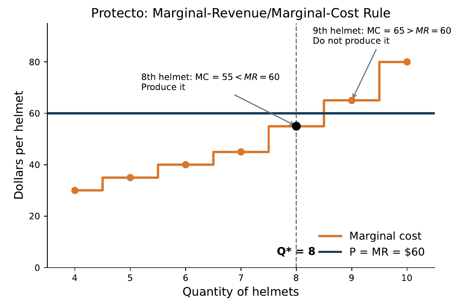
| Q | TR = 60Q | TC | \(\pi=TR-TC\) |
|---|---|---|---|
| 4 | 240 | 200 | 40 |
| 5 | 300 | 235 | 65 |
| 6 | 360 | 275 | 85 |
| 7 | 420 | 320 | 100 |
| 8 | 480 | 375 | 105 |
| 9 | 540 | 440 | 100 |
| 10 | 600 | 520 | 80 |
The table confirms that the largest profit among the listed quantities is $105 at 8 helmets.
Part E: Long-Run Market Adjustment
- Protecto and other firms are earning positive economic profit in the short run.
- In a perfectly competitive market, positive profit attracts new firms because entry is possible in the long run.
- Entry increases the number of sellers and shifts the market supply curve to the right.
- The rightward supply shift lowers the market equilibrium price.
- Entry continues until firms earn zero economic profit in long-run equilibrium, where price equals the minimum of average total cost for a representative firm.
Free Trade and a Tariff
Part A: Original Domestic Equilibrium
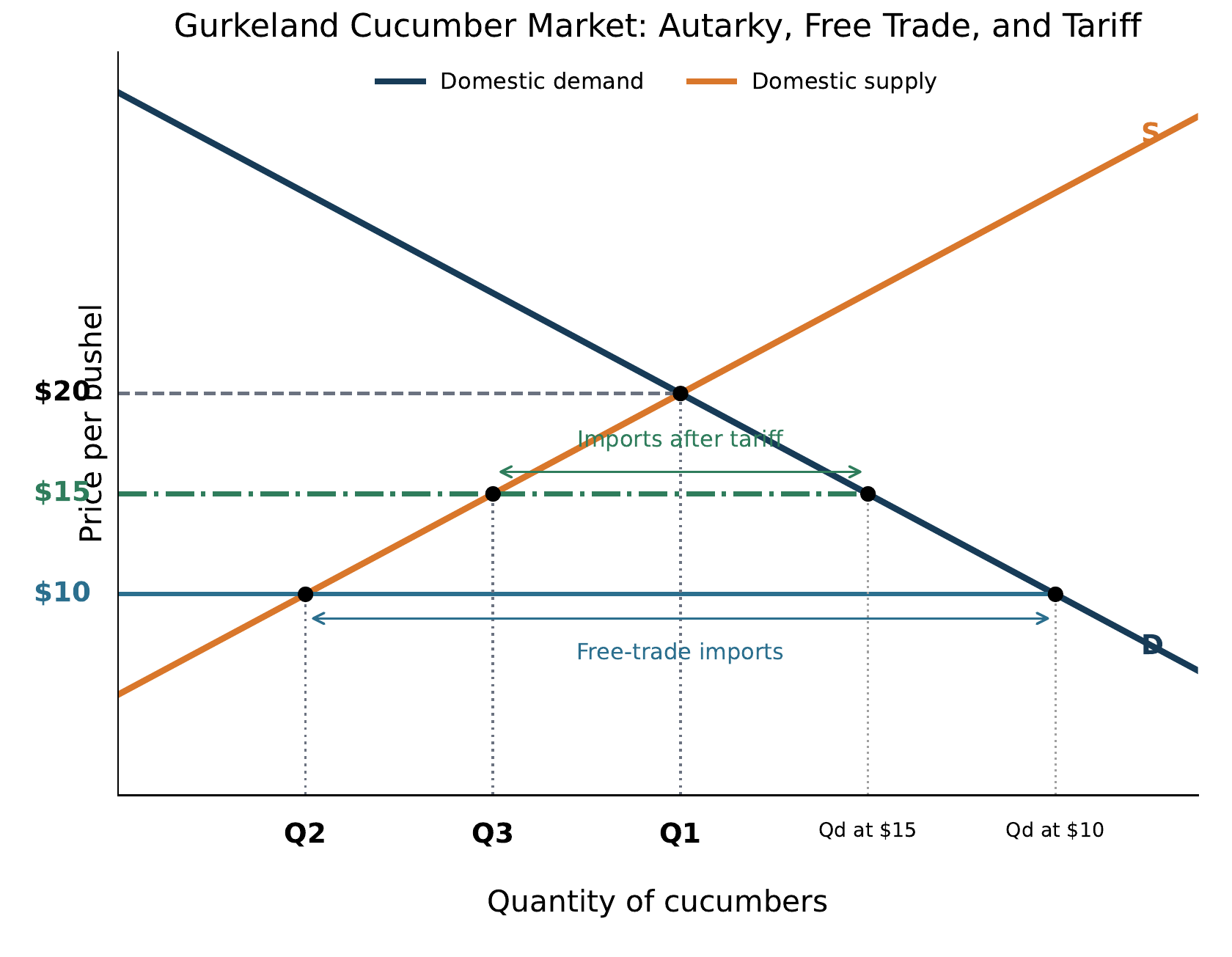
Part B(i): Free Trade at a World Price of $10
The world price is below the original domestic equilibrium price: \(\$10<\$20\). Under free trade, the domestic market price falls to $10. The quantity sold by domestic producers is found where the horizontal $10 line intersects the domestic supply curve. Label that quantity \(Q_2\). Because the lower price reduces domestic production, \(Q_2<Q_1\). Domestic consumers demand more than \(Q_1\) at $10; the gap between domestic quantity demanded and \(Q_2\) is filled by imports.
Part B(ii): Effect of Free Trade on Total Economic Surplus
The lower price transfers some surplus from domestic producers to consumers, but that transfer by itself does not change total surplus. Free trade also creates net gains:
- Consumers buy additional cucumbers whose willingness to pay exceeds the $10 world cost.
- Gurkeland stops producing some high-cost domestic units and imports them at the lower world price.
The gain in consumer surplus is larger than the loss in producer surplus. The difference is the gains from trade, represented by two welfare triangles in the standard trade diagram.
Part C(i): A $5 Tariff
For a small importing country, the tariff raises the domestic price by the amount of the tariff:
Find the intersection of the $15 horizontal line and the domestic supply curve. Label the quantity produced domestically as \(Q_3\). Since $15 lies between $10 and $20, the quantities satisfy \(Q_2<Q_3<Q_1\). Domestic production rises relative to free trade, while imports fall.
Part C(ii): Effect of the Tariff on Domestic Producer Surplus
The tariff raises the price received by domestic producers from $10 to $15. Producer surplus increases for two reasons:
- Producers receive a $5 higher price on the units they were already producing under free trade.
- The higher price makes additional domestic production profitable, so output expands from \(Q_2\) to \(Q_3\).
Graphically, the area above the domestic supply curve and below the market price becomes larger.
AP-Style Writing and Graphing Checklist
For Numerical Parts
- Write the equation first, such as \(AVC=(TC-FC)/Q\) or \(\pi=TR-TC\).
- Substitute the numbers visibly.
- State the final answer with units: dollars, dollars per helmet, helmets, or millions of dollars.
For Game-Theory Parts
- Use only the relevant player's payoff when comparing strategies.
- A dominant strategy must be best against every action of the other player.
- A Nash equilibrium requires mutual best responses in the same cell.
For Firm Graphs
- Label the vertical axis "Price and Cost" and the horizontal axis "Quantity."
- For monopoly, draw demand, MR, MC, and ATC; set output at MR = MC; obtain price from demand.
- Positive economic profit requires price above ATC at the profit-maximizing quantity.
- Deadweight loss lies between demand and MC from monopoly quantity to the efficient quantity.
For Trade Graphs
- Label domestic demand and supply, the original price $20, world price $10, and tariff-inclusive price $15.
- Label \(Q_1\) at the original equilibrium, \(Q_2\) at domestic supply under free trade, and \(Q_3\) at domestic supply after the tariff.
- State the direction first: total surplus increases with free trade; producer surplus increases with the tariff.
End of the detailed worked solutions. Prepared from the uploaded 2026 AP Microeconomics solution guide dated July 2026.