
Populations
APES Unit 3 Study Notes
Understand why populations grow and change.
Explore population growth, survivorship and human demographics with detailed notes, worked calculations and clear diagrams.
3.1 Generalist and Specialist Species
Overview
Species can be classified based on their niche breadth - the range of environmental conditions they can tolerate and resources they can utilize. Understanding whether a species is a generalist or specialist helps predict its vulnerability to environmental change, potential for invasiveness, and conservation needs. This concept directly relates to ecological tolerance (Unit 2.4) and population dynamics.
For the AP Environmental Science exam, you must be able to identify characteristics of each type, provide examples, and explain their advantages and disadvantages in different environmental contexts.
Generalist Species
Definition: Generalists use a relatively broad range of resources or habitats in the niche dimension being compared. A species can have a broad diet but narrow temperature tolerance. Eurytolerance describes broad tolerance of a specified abiotic factor; it is related to, but not identical with, generalism.
Characteristics of Generalist Species
- Broad Diet: Can eat many types of food (omnivores or varied diet within trophic level)
- Wide Habitat Range: Thrive in diverse environments and geographic areas
- Tolerance: Broad tolerance of some environmental conditions can accompany generalism, but a varied diet does not imply resistance to every temperature, pollutant or salinity.
- Behavioral Flexibility: Adapt behavior to changing conditions
- Large Geographic Distribution: Found across many regions and ecosystems
- Reproduction: Some successful generalists reproduce rapidly, while others mature slowly and invest heavily in offspring. Niche breadth and life-history strategy are different axes.
- Human-Associated: Many thrive in human-modified environments
Examples of Generalist Species
- Raccoons: Eat fruits, insects, fish, garbage; live in forests, wetlands, urban areas; active day or night
- Rats: Omnivorous diet; survive in diverse climates; highly successful in urban environments
- Coyotes: Eat rodents, fruits, carrion, garbage; adapt to forests, deserts, suburbs, cities
- White-tailed Deer: Browse on many plant species; habitat generalists
- Cockroaches: Some pest species eat varied foods and use buildings successfully. The group also contains habitat specialists, so do not generalize the traits of indoor pests to every cockroach species.
- Dandelions: Grow in many soil types and climates; reproduce prolifically
- Humans: Broad diets, cultural learning, technology and trade support occupation of diverse environments. This does not remove physiological limits or make every individual equally able to withstand all conditions.
- Crows: Omnivorous, intelligent problem-solvers, urban adapters
Advantages of Being a Generalist
- Resilience to Change: Can survive environmental disturbances and habitat alterations
- Resource Security: If one food source declines, can switch to alternatives
- Wide Distribution: Can colonize new areas and expand range
- Climate Change Resilience: Better able to adapt to changing conditions
- Lower Extinction Risk: Multiple survival strategies reduce vulnerability
- Invasive Potential: Can successfully establish in new environments
Disadvantages of Being a Generalist
- Potential trade-offs: Using several resources may involve compromises in efficiency or performance. Such trade-offs must be demonstrated for the species and resources compared, rather than assumed from the label generalist.
- Competition: A specialist may have an advantage on a particular resource in suitable conditions, but generalists are not inevitably outcompeted in every stable habitat.
- Resource efficiency: A specialist may use a particular resource more efficiently, but this is a potential trade-off to test, not proof that every generalist is less efficient on every resource.
- Costs of flexibility: Maintaining multiple physiological or behavioural responses may have costs, but a broad niche does not by itself prove higher energy use than a specialist.
Specialist Species
Definition: Specialists depend on a relatively narrow set of resources, habitats or conditions in the dimension assessed. A dietary specialist need not have narrow tolerance of every abiotic variable. Stenotolerance refers to a narrow range for a particular environmental factor.
Characteristics of Specialist Species
- Narrow Diet: Rely on one or few food sources (often obligate relationships)
- Specific Habitat Requirements: Need particular temperature, moisture, vegetation, or geographic features
- Low Tolerance: Sensitive to environmental changes (pollution, temperature shifts, habitat disturbance)
- Limited Distribution: Restricted to specific regions or ecosystems
- Specialized traits: Adaptations can suit a particular resource or habitat. Specialist species are not “more evolved” than generalists; all present-day lineages have evolutionary histories.
- Reproductive rate: Some specialists reproduce slowly, but specialized insects can have many offspring and short generations. Specialization does not define r- or K-associated traits.
- Indicator use: A species with a known response can help indicate a specified environmental condition. Not every specialist is a validated indicator, and absence may reflect dispersal or habitat as well as pollution.
Examples of Specialist Species
- Giant Pandas: Eat almost exclusively bamboo (99% of diet); require bamboo forests in specific mountain ranges in China
- Koalas: Feed mainly on leaves from selected eucalyptus species and depend on suitable woodland. Their dietary specialization does not mean every eucalyptus species is equally usable or that no other food is ever consumed.
- Polar bears: Depend strongly on sea ice for access to seal prey. Sea-ice loss changes feeding opportunities and energetics; the concern is not simply an absolute inability to survive any warmer air temperature.
- Spotted Owls: Require old-growth forests with dense canopy in Pacific Northwest
- Monarch Butterflies: Caterpillars feed exclusively on milkweed plants
- Corals: Many shallow tropical reef-building corals depend on appropriate light, temperature, salinity and water quality. Deep and cold-water corals also exist, so “all corals require warm shallow water” is incorrect.
- Snail Kite: Feeds almost exclusively on apple snails in Florida wetlands
- Trout: Require cold, clean, well-oxygenated water; sensitive to temperature increases and pollution
Advantages of Being a Specialist
- Reduced Competition: Specialized niche means fewer competitors for specific resources
- Optimal Efficiency: Highly efficient at exploiting their particular resource or habitat
- Stable Environments: Excel when conditions remain constant and predictable
- Unique Adaptations: Specialized traits allow access to resources generalists cannot use
- Access to a niche: Specialized traits can provide access to resources less usable by other species; this does not guarantee a monopoly or absence of competitors.
Disadvantages of Being a Specialist
- Vulnerable to Change: Environmental disturbances or habitat loss can be catastrophic
- Resource Dependency: If specialized food/habitat disappears, species cannot easily adapt
- High Extinction Risk: Especially vulnerable to climate change, habitat fragmentation, pollution
- Limited Range Expansion: Cannot colonize new areas that lack specific requirements
- Conservation: Specialization can increase risk when a required resource or habitat declines, but specialist status alone does not mean a species is endangered or requires the same conservation intervention as another species.
- Climate Change Vulnerability: Cannot easily shift ranges or adapt to new conditions
⚠️ Common Pitfall: Don't confuse generalists/specialists with r/K selection (next topic)! They're related but different concepts. Generalists CAN have K-selected traits (elephants are generalist feeders but K-selected). Specialists CAN have r-selected traits (some specialized insects). The key distinction: generalist/specialist describes NICHE BREADTH; r/K describes REPRODUCTIVE STRATEGY.
Apply niche breadth to a changed habitat
Worked reasoning: A bird eating several seed and insect types may be less affected by the loss of one food than a bird depending on that food during breeding. This is a prediction about the stated diet and season, not proof of broad tolerance to every pollutant or climate condition. Generalists can still decline when all suitable habitat disappears.
Keep categories separate: An elephant can be a generalist feeder and have slow reproduction; a host-specific insect can be a specialist and reproduce rapidly. Describe niche breadth, generation time, offspring production and parental investment separately before predicting recovery or invasion risk.
3.2 K-Selected and r-Selected Species
Overview
r/K selection theory is a simplified framework contrasting rapid potential increase with traits favouring persistence under crowding. In the logistic equation, r is a per-capita rate parameter and K is carrying capacity. Species often combine traits from both ends; modern life-history analysis also examines survival, reproductive timing and trade-offs directly. Learn the AP comparison as a model rather than a universal classification.
For the AP Environmental Science exam, you must understand the characteristics, advantages, environments, and examples of each strategy. This concept is critical for understanding population dynamics, conservation, and invasive species.
r-Selected Species (Opportunists)
Definition: The r-associated end of the comparison emphasizes early reproduction, short generations and many relatively low-investment offspring. These traits can aid colonization when conditions permit rapid increase. They do not imply that offspring have lower biological “quality,” or that environmental conditions are always unpredictable.
Characteristics of r-Selected Species
- High Reproductive Rate: Produce many offspring in short time periods
- Small Body Size: Typically small organisms (though not always)
- Early Sexual Maturity: Reproduce at young ages
- Short Life Span: Live fast, die young strategy
- Little/No Parental Care: Offspring fend for themselves immediately after birth
- High Mortality Rate: Most offspring die before reproducing
- Rapid Development: Fast growth to maturity
- Opportunistic: Exploit temporary resources and favorable conditions quickly
- Population Fluctuations: Experience boom-and-bust cycles
- Mortality: Density-independent disturbances can strongly affect these populations, but competition, disease and other density-dependent processes can also limit them. A reproductive strategy does not determine the only source of mortality.
Examples of r-Selected Species
- Insects: Many mosquitoes, flies and aphids have short generations and high reproductive potential. Fecundity and parental care vary across insects; thousands of eggs is not a fixed value for every individual or species.
- Bacteria: Reproduce exponentially under favorable conditions
- Weeds: Dandelions, crabgrass (prolific seed production)
- Mice and Rats: Multiple litters per year, many offspring per litter
- Many fishes: Cod can release very large numbers of eggs; salmon commonly produce thousands rather than millions per female. Some fish provide parental care. Use the species and reproductive system specified rather than a single rule for all fishes.
- Frogs: Lay hundreds to thousands of eggs in water
- Annual Plants: Complete life cycle in one season, produce many seeds
- Oysters: Can produce millions of larvae
Environmental Conditions Favoring r-Selection
- Unstable/Unpredictable: Environments subject to frequent disturbances
- Early Succession: Recently disturbed or colonized areas
- Variable Resources: Resource availability fluctuates dramatically
- Low Competition: Populations well below carrying capacity
- Short Growing Seasons: Must reproduce quickly before conditions deteriorate
Advantages of r-Selection Strategy
- Can rapidly colonize new or disturbed habitats
- Exploit temporary resource abundances quickly
- High probability that some offspring survive unpredictable conditions
- Rapid population recovery after disturbances
- Effective in pioneer/early successional stages
K-Selected Species (Equilibrium Species)
Definition: The K-associated end commonly includes delayed maturity, long life and relatively low reproductive output. Large mammals often invest heavily in offspring, but long-lived plants and some reptiles combine slow adult life histories with many seeds or eggs and little post-release care. These traits do not guarantee a population stays exactly at K.
Characteristics of K-Selected Species
- Low Reproductive Rate: Produce few offspring, often one at a time
- Large Body Size: Typically larger organisms (though not always)
- Late Sexual Maturity: Reproduce only after reaching older ages
- Long Life Span: Live for many years or decades
- Extensive Parental Care: Parents invest heavily in protecting and nurturing offspring
- Low Mortality Rate: High offspring survival due to parental care
- Slow Development: Extended juvenile period with learning and growth
- Competitive: Strong competitors in stable environments
- Population variation: Some populations fluctuate near resource limits, while others change because of harvest, disease, climate or migration. A K-associated life history is not proof of a stable population size.
- Density-Dependent Mortality: Death often due to competition and predation
Examples of K-Selected Species
- Large Mammals: Elephants, whales, gorillas, humans (1-2 offspring, years of care)
- Large Birds: Eagles, albatross, condors (1-2 eggs, extended parental care)
- Sharks: Many species mature late and have relatively low reproductive output, with some investing substantially before birth or hatching. Post-birth parental care is generally absent; shark reproductive modes and fecundity vary.
- Trees: Oaks, redwoods and sequoias illustrate long adult lives and delayed reproduction, yet can produce many seeds with high early mortality. This shows why slow adult life history and Type III early survivorship can coexist.
- Bears: 1-3 cubs every 2-3 years, extensive maternal care
- Primates: Chimpanzees, orangutans (single births, years of dependency)
- Tortoises: Long-lived, slow reproduction
- Large Predators: Lions, tigers, wolves (small litters, extended care)
Environmental Conditions Favoring K-Selection
- Stable/Predictable: Consistent environmental conditions over time
- Late Succession/Climax: Mature, established ecosystems
- Constant Resources: Reliable resource availability year-round
- High Competition: Populations at or near carrying capacity
- Low Disturbance: Infrequent environmental disruptions
Advantages of K-Selection Strategy
- High offspring survival rate due to parental investment
- Better competitors in stable, resource-limited environments
- Offspring better equipped with learned behaviors and skills
- Maintain stable populations in climax communities
- Long lifespan provides multiple reproductive opportunities
r vs. K Comparison Table
| Characteristic | r-Selected Species | K-Selected Species |
|---|---|---|
| Number of Offspring | Many | Few |
| Parental Care | Little to none | Extensive |
| Maturation Time | Fast/Early | Slow/Late |
| Life Span | Short | Long |
| Body Size | Usually small | Usually large |
| Population Size | Variable (boom/bust) | May persist near resource limits; can fluctuate |
| Environment | Unstable/Unpredictable | Stable/Predictable |
| Competition | Low | High |
| Succession Stage | Early (pioneer) | Often associated with established communities |
| Mortality | Both types can be affected; disturbance often important | Both types can be affected; crowding often important |
Exam tip: Compare actual traits and recognize a continuum. Rapid reproduction can aid spread, while slow reproduction can delay recovery after losses. Invasive species also include long-lived organisms, and endangered status is not determined by r/K traits alone. Distinguish potential reproduction from realized population growth under current conditions.
Use several traits before drawing a conclusion
A long-lived tree may produce thousands of seeds and lose most seedlings, while its surviving adults persist for centuries. A mammal may produce relatively few young with prolonged care. Seed number alone therefore cannot assign every organism to one life-history endpoint. The comparison table summarizes typical associations, not a set of necessary conditions.
Conservation application: If a hypothetical animal first breeds at age 12 and produces one offspring every three years, adult mortality can be difficult to offset quickly. Protecting adult survival and habitat can matter as much as increasing births. High fecundity elsewhere does not guarantee recovery when habitat or early survival remains limiting.
3.3 Survivorship Curves
Overview
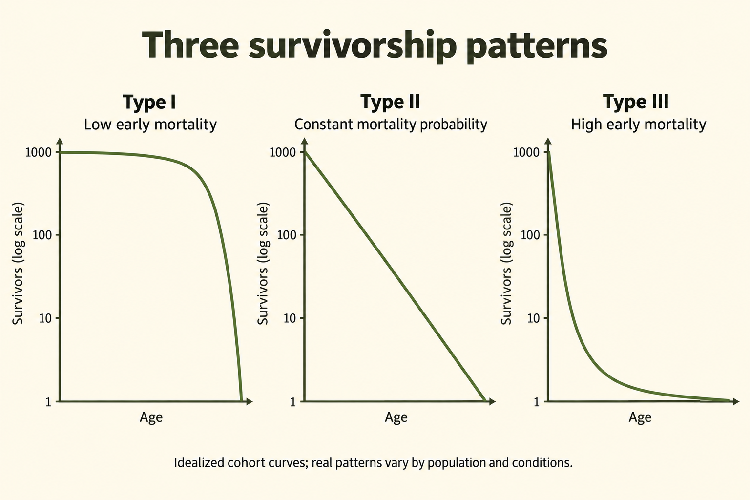
Survivorship curves are graphs that show the proportion or percentage of individuals surviving at each age in a population. They provide visual representations of mortality patterns across a species' lifespan and help ecologists understand life history strategies. The x-axis represents age or percentage of maximum lifespan, while the y-axis represents the number or percentage of survivors (typically on a logarithmic scale).
For the AP Environmental Science exam, you must be able to identify and interpret the three types of survivorship curves, explain what they reveal about reproductive strategies, and provide examples of species for each type.
Type I Survivorship Curve (Low Early Mortality)
Characteristics
Pattern: High survival rates throughout early and middle life, with mortality concentrated in older age groups. The curve stays relatively flat (high survival) until late in life, then drops steeply.
Shape: High early survivorship followed by a steep late-life decline. Describe where mortality occurs rather than rely on ambiguous “convex/concave” labels; the displayed shape also depends on the axis scale.
Mortality Pattern: Most individuals survive to old age and die from aging-related causes. Very few die young.
Life History Strategy: Strongly associated with K-selected species
Key Features
- High Parental Investment: Extensive care and protection of offspring
- Few Offspring: Low reproductive output per breeding event
- High Infant Survival: Most young survive to adulthood
- Long Lifespan: Individuals live many years
- Late Sexual Maturity: Begin reproducing at older ages
- Death Cause: Primarily senescence (aging) and age-related diseases
Examples
- Humans (developed countries with modern healthcare)
- Large Mammals: Elephants, whales, gorillas, rhinoceros
- Large Birds: Eagles, albatrosses, swans
- Domestic Animals: Well-cared-for pets, livestock
- Some Marine Mammals: Dolphins, orcas
Interpretation: A Type I pattern shows relatively low mortality early and in midlife, followed by greater late-life mortality. Parental care and protected conditions can contribute, but the curve alone does not prove the cause of death, guarantee survival to a fixed maximum age or specify offspring number.
Type II Survivorship Curve (Constant Mortality)
Characteristics
Pattern: Relatively constant mortality rate throughout life. Individuals have approximately equal probability of dying at any age.
Shape: A straight declining line when survivorship is on a logarithmic y-axis and age on a linear x-axis. With a linear survivorship axis, constant mortality probability gives an exponential decline, not a straight line.
Mortality pattern: Approximately the same probability of dying per individual per unit time across the ages considered. Equal proportions, rather than equal numbers of the original cohort, die in successive intervals.
Life History Strategy: Intermediate between r and K selection
Key Features
- Moderate Parental Care: Some protection but not extensive
- Moderate Offspring Number: Neither extremely high nor low reproduction
- Equal Vulnerability: Young, middle-aged, and old face similar mortality risks
- Random Death: Mortality often due to unpredictable events (accidents, predation, disease)
- Possible causes: Predation, disease or other hazards may contribute. A roughly constant age-specific probability does not show that one particular cause acts equally on every individual.
Examples
- Many Birds: Songbirds, robins, gulls
- Small Mammals: Squirrels, rabbits, mice (in wild populations)
- Some Reptiles: Lizards, some snakes
- Rodents: Prairie dogs, chipmunks
- Some Invertebrates: Hydra, certain mollusks
Interpretation: Type II is an idealized age pattern with approximately constant mortality probability across the interval studied. Real populations may approximate it over part of their lives. A survivorship curve describes outcomes; it does not by itself establish that deaths are random or identify the mechanism.
Type III Survivorship Curve (High Early Mortality)
Characteristics
Pattern: Very high mortality in early life stages, but individuals that survive to adulthood have high survival rates thereafter. The curve drops steeply at first, then levels off.
Shape: A steep early drop followed by a flatter later portion: many individuals die young, while survivors experience lower subsequent mortality over the ages considered.
Mortality Pattern: Most individuals die very young (often >90% mortality in juvenile stages). Those that reach adulthood tend to survive longer.
Life History Strategy: Strongly associated with r-selected species
Key Features
- No/Minimal Parental Care: Offspring left to fend for themselves immediately
- Many Offspring: Extremely high reproductive output
- Low Infant Survival: Vast majority die before maturity
- Vulnerable Young: Juveniles are easy prey or susceptible to environmental stresses
- Many-offspring strategy: High reproductive output can offset low early survival over generations, although it does not guarantee persistence when all suitable habitat or recruitment conditions are lost.
- Death Cause: Predation, starvation, environmental conditions affect young; adults die from various causes
Examples
- Many fishes: Species with high egg or larval mortality can show Type III-like patterns. Egg output and survival differ widely; do not assume every salmon, cod or tuna produces millions of eggs or shares one exact survival percentage.
- Marine Invertebrates: Oysters, sea urchins, corals (broadcast spawning)
- Insects: Many have high egg or larval mortality, but reproductive output and parental protection vary. Social insects and species that guard offspring illustrate why one curve or egg count cannot describe all insects.
- Amphibians: Frogs, toads (hundreds of eggs, few tadpoles survive)
- Plants: Most species (thousands of seeds, few germinate and reach maturity)
- Sea Turtles: Lay many eggs on beaches; hatchlings face extreme predation
- Many Invertebrates: Spiders, crustaceans
Interpretation: Type III curves indicate species that produce vast numbers of offspring with minimal investment in each. This "numbers game" strategy compensates for extremely high juvenile mortality. Common in species that reproduce in unpredictable environments, have many predators, or whose young must disperse widely.
Survivorship Curve Comparison
| Feature | Type I | Type II | Type III |
|---|---|---|---|
| Curve Shape | Late-life decline | Straight on log-survivorship axis | Early decline, then flatter |
| Early Mortality | Very Low | Moderate | Very High |
| Parental Care | Extensive | Moderate | Little/None |
| Offspring Number | Few | Moderate | Many |
| Selection Type | Often associated; not a rule | Intermediate | Often associated; not a rule |
| Death Timing | Old age | Similar per-individual probability per interval | Young age |
| Examples | Humans, elephants | Birds, rodents | Fish, insects, plants |
Common pitfall: Read axes first. Type I concentrates mortality late, Type II has roughly constant mortality probability and Type III concentrates it early. Type II is straight on semilog axes, not necessarily on linear axes. Life-history associations are tendencies, not identities: a long-lived tree can show high seedling mortality.
Calculate survivorship and mortality from a cohort
Cohort: Track a group born or established during the same interval. If 1,000 individuals begin and 800 are alive one year later, survivorship to age 1 is The interval mortality proportion is If 640 survive the following year, the second interval mortality proportion is Both intervals have 20% mortality, even though deaths fall from 200 to 160.
Scale check: With constant 20% mortality per year, survivors follow . On a logarithmic axis this is a straight decline; on a linear axis it bends. Log axes cannot include zero. A survival curve follows the original cohort and does not add newborns to it, unlike a graph of total population size.
3.4 Carrying Capacity
Overview
Carrying capacity (K) is a model of the population size that specified environmental conditions and resources can sustain over time. In the basic closed logistic model, net growth is zero at because births and deaths balance. With migration, zero total change instead requires births + immigration = deaths + emigration. K depends on species, habitat, resource renewal and time; it is not simply the largest observed count.
For the AP Environmental Science exam, you must understand factors that determine carrying capacity, how populations respond when they exceed K, and the difference between carrying capacity for different species and for humans.
Factors Determining Carrying Capacity
Limiting Resources
- Food Supply: Availability and quality of nutrition sources
- Water: Access to clean, fresh water
- Space/Territory: Physical area for living, breeding, and foraging
- Shelter: Protection from weather and predators (nesting sites, den locations)
- Light: For plants and photosynthetic organisms
- Nutrients: Minerals and chemical elements (nitrogen, phosphorus for plants)
Environmental Factors
- Climate: Temperature and precipitation patterns
- Habitat Quality: Condition and suitability of the environment
- Predation: Pressure from predators
- Disease: Prevalence of pathogens and parasites
- Competition: Both intraspecific (within species) and interspecific (between species)
- Waste Accumulation: Toxic waste products that inhibit growth
Density-Dependent Factors
Density-dependent effects change in strength with population density, often reducing per-capita growth as crowding rises. Such feedback can regulate populations, but does not hold every real population exactly at a fixed K. Identify the mechanism rather than assume every disease or predator response is strictly density-dependent.
- Competition for Resources: More individuals = more competition for limited food, water, space
- Predation: Higher prey density makes hunting easier for predators
- Disease Transmission: Pathogens spread more easily in crowded populations
- Parasitism: Higher host density increases parasite transmission
- Stress: Crowding increases physiological stress, reducing reproduction and survival
- Waste Buildup: Toxic metabolic waste accumulates in high-density areas
Population Dynamics at Carrying Capacity
At Carrying Capacity ()
- Zero net growth: In the closed model, births balance deaths. An open population can have births unequal to deaths while migration offsets the difference.
- Stable Population Size: Number of individuals remains relatively constant
- Resource Balance: Resources are being consumed at the rate they're replenished
- Maximum Sustainable Population: Highest number that can persist long-term
Above Carrying Capacity () - Overshoot
When a population temporarily exceeds carrying capacity:
- Resource Depletion: Consumption exceeds regeneration rate
- Environmental Degradation: Habitat damage reduces future carrying capacity
- Increased Mortality: Starvation, disease, stress cause death rates to rise
- Decreased Reproduction: Stressed individuals have fewer offspring
- Possible decline: Overshoot can lead to mortality, reduced reproduction or emigration. Delays in feedback can produce a crash or oscillation, and habitat degradation can lower later K. An immediate crash below K is possible, not inevitable after every overshoot.
Example: Deer populations without predators can overshoot carrying capacity, overgraze vegetation, damage habitat, then crash from starvation.
Below Carrying Capacity ()
- Resources: In the simple model, lower crowding leaves greater resources per individual. Below an estimated K does not guarantee that every nutrient, breeding site or seasonal resource is abundant.
- Low Competition: Reduced intraspecific competition
- Growth tendency: The basic logistic model with positive r predicts increase for 0 < . Real populations can still decline because of harvest, severe weather, emigration or difficulty finding mates at low density.
- Trend: Population increases toward K
Changes in Carrying Capacity
Carrying capacity is dynamic and can change over time:
Factors That INCREASE Carrying Capacity
- Increased food supply (better rainfall, more prey)
- Habitat expansion or restoration
- Reduction in predators or competitors
- Improved environmental conditions (favorable climate)
- Disease control or eradication
- For humans: Agricultural technology, medicine, sanitation, resource extraction
Factors That DECREASE Carrying Capacity
- Habitat destruction or degradation
- Resource depletion (overfishing, deforestation)
- Pollution and environmental contamination
- Climate change altering suitable habitat
- Introduction of competitors, predators, or diseases
- Drought or natural disasters
- Fragmentation reducing effective habitat area
Human Carrying Capacity
Estimating Earth's carrying capacity for humans is complex and controversial because:
- Technology and health: Agriculture, infrastructure and medicine have enabled larger populations and changed survival and resource access. Population support and long-term ecological sustainability are different questions; finite inputs, waste, soil condition and consumption still constrain outcomes.
- Variable Consumption: Carrying capacity depends on lifestyle and resource use per person (developed vs. developing nations)
- Resource Substitution: Humans can switch between resources and develop alternatives
- Delayed Feedback: Effects of overshoot may not appear for generations
- Non-Renewable Resources: Humans use finite resources (fossil fuels, minerals) that don't regenerate
Key Question: Are we above, at, or below Earth's carrying capacity for humans?
Arguments vary based on assumptions about technology, consumption patterns, and what quality of life constitutes "sustainable." Signs of potential overshoot include: resource depletion, biodiversity loss, climate change, ocean acidification, and ecosystem degradation.
Exam tip: Distinguish sustainable support from a temporary count. K can change; populations can overshoot and later decline, oscillate or approach a new equilibrium. Use the stated assumptions and response times. Do not infer one fixed global human carrying capacity from population size alone.
Density-dependent and density-independent effects
Density-dependent example: As a deer population becomes crowded, forage per animal falls and reproduction declines. Density-independent example: A severe freeze can kill plants without being caused by their density. The consequences can still interact with density: crowded or poorly nourished animals may recover less readily from a storm.
Changing K: Suppose a site could support about 800 animals under prior conditions, but drought reduces forage and the estimated K falls to 500. A count of 650 is now above the new estimate, even if it was below the former one. Predict the mechanism and uncertainty rather than assert that 150 animals must die immediately.
3.5 Population Growth and Resource Availability
Overview
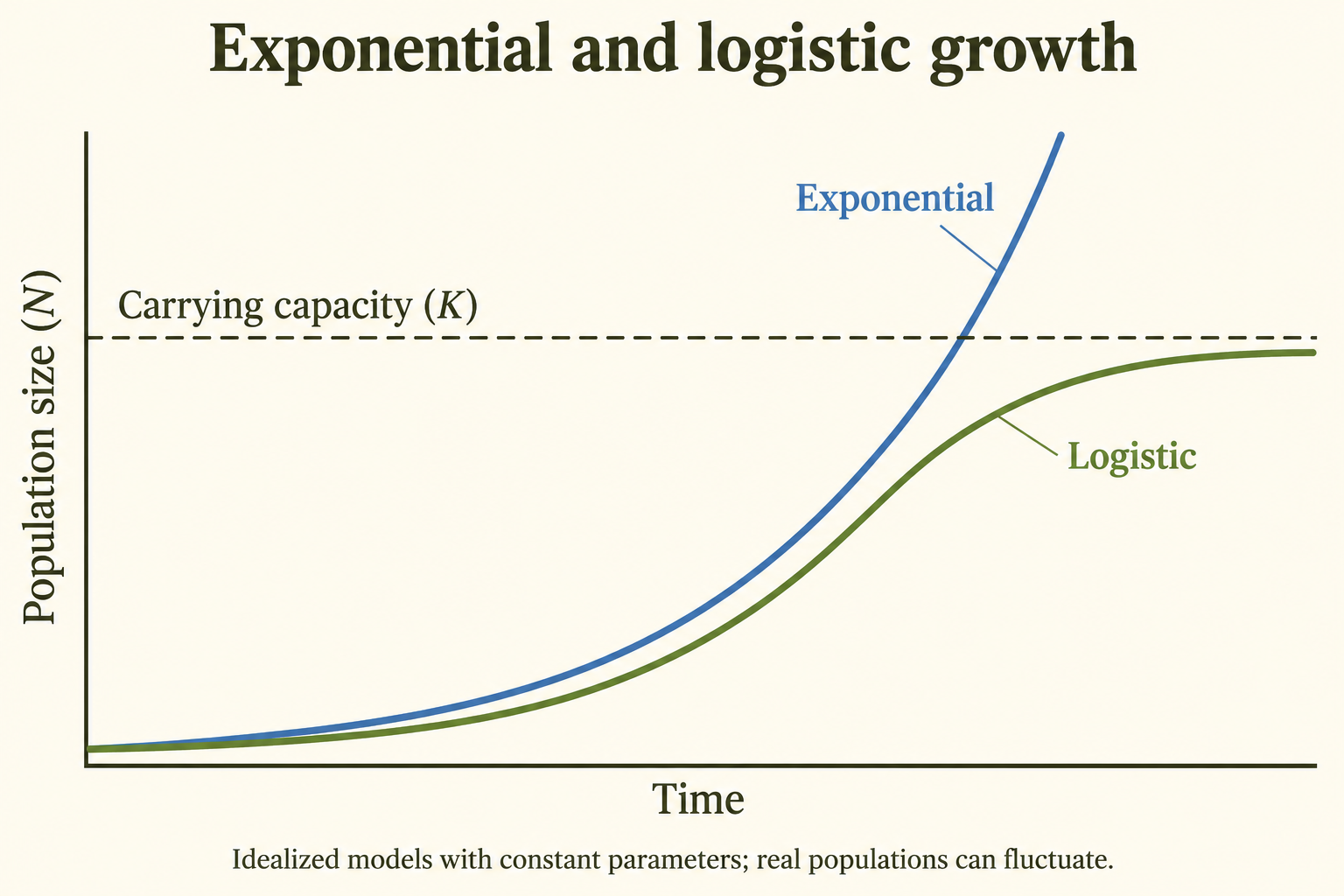
Population growth patterns are fundamentally linked to resource availability. Understanding how populations grow - and what limits that growth - is central to environmental science. Two primary growth models describe population dynamics: exponential growth (J-curve) and logistic growth (S-curve).
For the AP Environmental Science exam, you must understand both growth models, recognize their equations, interpret graphs, and explain the factors that cause transitions between growth patterns.
Exponential Growth (J-Curve)
Characteristics
Definition: Exponential growth assumes a constant positive per-capita rate r, so total increase is proportional to current N. It can approximate a period with weak density limitation; it does not require literal absence of every predator or death. The intrinsic maximum rate under ideal conditions is often written .
Pattern: Population size increases slowly at first, then faster and faster as the population grows larger. The larger the population, the faster it grows (positive feedback loop).
Shape: J-shaped curve - starts flat, then curves upward steeply
Exponential Growth Equation
Where:
- = instantaneous rate of change of population size with respect to time
- = intrinsic growth rate (per capita rate of increase)
- = population size
Key Point: Growth rate is proportional to population size. As N increases, growth rate increases proportionally. This is why the curve gets steeper over time.
Conditions for Exponential Growth
- Unlimited Resources: Abundant food, water, space, shelter
- Ideal Environmental Conditions: Optimal temperature, moisture, pH
- Mortality: Predation or disease need not be zero. The model requires a roughly constant net per-capita rate over the interval; it fails when those effects cause substantial density-dependent or time-varying changes.
- No Competition: Population well below carrying capacity
- Migration assumption: The basic rN equation is commonly applied to a closed population. In an open system, include immigration and emigration explicitly, or explain how they enter the model.
When Exponential Growth Occurs
- Colonization: Species entering a new habitat with no competition
- Recovery: Population rebounding after a major decline
- Temporarily: After disturbance clears area (fire, flood)
- Laboratory Cultures: Bacteria in fresh nutrient broth
- Invasive Species: Non-native species in new environments without natural predators
- Human Population: Historically experienced near-exponential growth with agriculture and technology
Limitations of Exponential Growth
Critical Point: Exponential growth cannot continue indefinitely in nature. Eventually, limiting factors (resource depletion, waste accumulation, disease, predation) slow growth.
Reality: Positive exponential increase cannot continue indefinitely with finite resources. Growth may later slow, reverse, oscillate or be interrupted by disturbance; populations do not have to follow one smooth logistic curve afterward.
Logistic Growth (S-Curve)
Characteristics
Definition: Population growth that slows as the population approaches carrying capacity (K). Growth is initially exponential but decelerates as resources become limited, eventually stabilizing at K.
Pattern: S-shaped (sigmoidal) curve with three phases:
- Early phase: When N is small, total additions can be small even with a high per-capita rate. A biological lag is not an extra feature required by the basic logistic equation.
- Exponential/Log Phase: Rapid growth (abundant resources, low competition)
- Stationary/Plateau Phase: Growth slows and stabilizes at carrying capacity
Shape: S-shaped curve - slow start, steep middle, levels off at top
Logistic Growth Equation
Where:
- = instantaneous rate of change of population size with respect to time
- = intrinsic growth rate
- = current population size
- = carrying capacity
- : A dimensionless density-limitation term in the model. It is not a measured fraction of physical space or of every resource remaining. It equals and becomes negative when .
Key Point: The term is the key difference from exponential growth:
- When N is small, , so growth is approximately exponential
- As N approaches K, approaches 0, so growth slows
- When , , so growth stops ()
When Logistic Growth Occurs
- Natural populations: Some populations approximate logistic growth over a particular period. Fluctuating resources, age structure, time lags, migration and stochastic events often cause departures from the ideal S-curve.
- Resource Limitation: When food, space, or other resources become scarce
- Stable Environments: Mature ecosystems near carrying capacity
- Density-Dependent Regulation: Competition, predation, disease increase with density
- K-Selected Species: Populations adapted to crowded conditions
Factors That Slow Growth at K
- Resource Competition: Insufficient food/water/space for all individuals
- Increased Predation: Higher prey density attracts more predators
- Disease Spread: Pathogens transmit more easily in crowded populations
- Stress: Crowding causes physiological stress, reducing reproduction
- Territoriality: Dominant individuals exclude others from breeding
- Waste Accumulation: Toxic metabolites inhibit growth
Exponential vs. Logistic Growth Comparison
| Feature | Exponential Growth | Logistic Growth |
|---|---|---|
| Curve Shape | J-shaped | S-shaped |
| Growth Rate | Accelerates continuously | Slows as N approaches K |
| Resources | Unlimited | Limited |
| Carrying Capacity | Not reached | Approached under fixed model assumptions |
| Equation | ||
| Sustainability | Unsustainable | Equilibrium at K in the basic model |
| Competition | Minimal | Significant |
| Real-World | Temporary, rare | Useful approximation; real populations can fluctuate |
Common pitfall: is an instantaneous rate, while is an average over a finite interval. For the basic logistic model with fixed positive and , the total growth rate is highest at ; per-capita growth is highest at low . At , net growth is zero while births and deaths continue. Real populations need not follow the ideal curve exactly.
Worked growth rates, units and a population budget
Exponential: Let organisms and . The instantaneous rate is Over a full year with continuous constant , use This gives Simply adding 100 is an initial-rate approximation, not the exact continuous solution.
Logistic: With the same and and , At the rate is ; at it is zero. For these parameters the maximum total rate is
Open-population budget: Over a stated year, births , deaths , immigrants and emigrants . Net change is An initial population of 1,000 ends at 1,060: a 6% increase. Keep counts, per-capita rates and percentages distinct.
3.6 Age Structure Diagrams
Overview
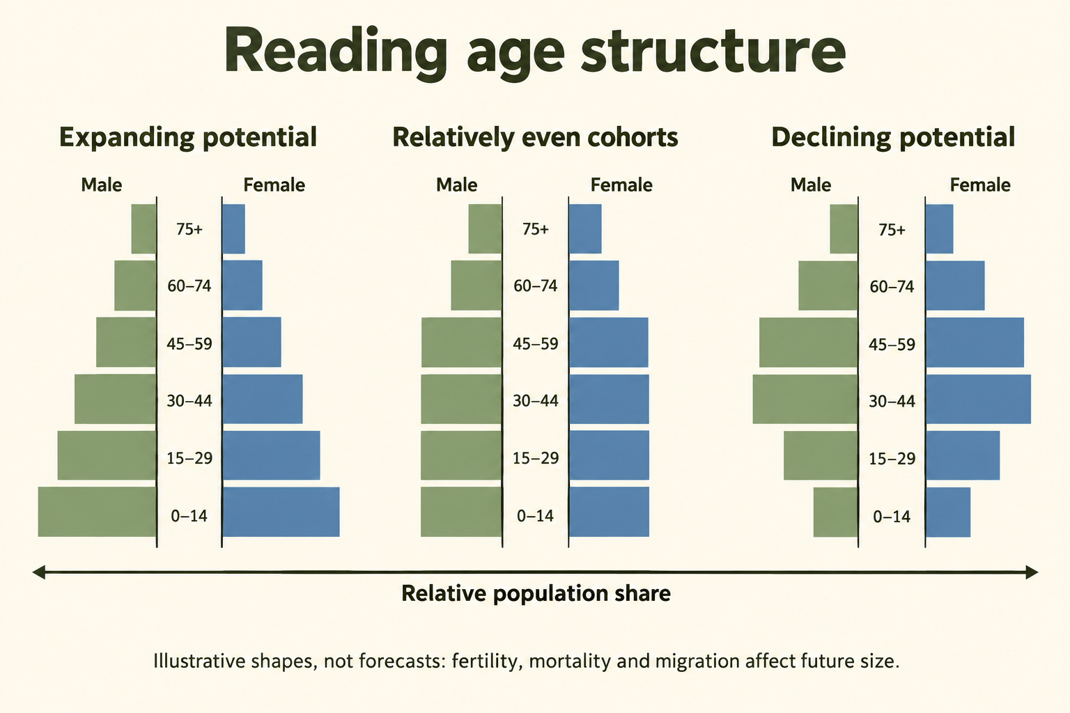
Age structure diagrams show the distribution of a population among age groups, often separated by sex. Shape helps explain population momentum and service needs, but future size also depends on fertility, mortality and migration. Read the date, cohort widths and whether bars show counts or percentages before comparing populations.
For the AP Environmental Science exam, you must be able to interpret age structure diagrams, predict future population trends, and understand how age structure relates to economic development, resource needs, and social services.
Structure of Age Structure Diagrams
Components
- Horizontal Axis: Percentage or number of individuals in each age group
- Vertical Axis: Age groups (typically 5-year cohorts: 0-4, 5-9, 10-14, etc.)
- Left Side: Males (conventionally)
- Right Side: Females (conventionally)
- Bottom (Wide Base): Young population (pre-reproductive age: 0-14 years)
- Middle: Reproductive age adults (15-44 years)
- Top (Narrow): Older population (post-reproductive age: 45+ years)
Three Key Age Groups
- Pre-reproductive grouping (often 0–14): A simplified classroom category for younger cohorts. It is not a claim that no individual can reproduce before age 15.
- Reproductive grouping (often 15–44 in AP diagrams): A simplified age band; demographic fertility statistics commonly use ages 15–49. Actual reproductive timing varies, and births depend on age-specific fertility and the number of people in relevant cohorts.
- Older grouping (often 45+ in simplified diagrams): A study category rather than a universal biological boundary. People aged 45–64 may still be working or reproducing; do not confuse this category with the 65+ band used in many dependency ratios.
Types of Age Structure Diagrams
Rapid Growth (Expanding) Pyramid
Shape: Wide base (pyramid shape) - many young people, fewer old people
Indicates: A relatively large younger cohort, often associated with high recent births. Life expectancy and mortality cannot be established from the base width alone.
Prediction: A large younger cohort can create positive momentum as it ages, if fertility, mortality and migration do not offset it. A broad base alone does not prove a fixed future growth rate or low life expectancy.
Characteristics:
- Large proportion (>35%) under age 15
- Small proportion (<5%) over age 65
- High fertility rate (>3 children per woman)
- High infant mortality rate
- Short life expectancy
Illustrative contexts: Nigeria, Afghanistan, Niger, the Democratic Republic of the Congo and Mali have often been used to discuss youthful age structures. Use a dated pyramid rather than assume every country at a similar income level has the same shape or rate of growth.
Economic/Social Implications:
- Need for schools, education, child healthcare
- High dependency ratio (many dependents per working adult)
- Future job creation challenges as youth enter workforce
- Potential for rapid population momentum
Slow Growth (Stationary) Column
Shape: Relatively uniform width (column or box shape) - similar numbers across age groups
Indicates: Low birth rate, low death rate, long life expectancy, stable population
Prediction: Relatively similar younger and middle cohorts can be consistent with slow growth, but do not prove exact stability or replacement fertility. Future age-specific rates and migration still matter.
Characteristics:
- Moderate proportion (~20-25%) under age 15
- Growing proportion (10-15%) over age 65
- Fertility rate near replacement level (~2.1 children per woman)
- Low infant mortality
- High life expectancy
Illustrative contexts: The United States, Canada and Australia have experienced ageing and substantial migration. Their exact age profiles vary by year. China should not be treated as a permanent stable-column example; low fertility and ageing have changed its structure.
Economic/Social Implications:
- Balanced dependency ratio
- Aging population requiring increased healthcare
- Stable workforce
- Social security and pension sustainability concerns
Negative Growth (Declining) Inverted Pyramid
Shape: Narrow base, wider middle/top (inverted pyramid or urn shape) - fewer young, more elderly
Indicates: Very low birth rate, very low death rate, very long life expectancy, aging population
Prediction: Fewer young people than in recent adult cohorts can indicate low recent births and potential natural decrease later. Total population can still increase with net immigration; use the rates and age distribution together.
Characteristics:
- Small proportion (<15-18%) under age 15
- Large proportion (>15-20%) over age 65
- Fertility rate well below replacement (<1.5-2.0 children per woman)
- Very low infant mortality
- Very high life expectancy (>80 years)
Illustrative contexts: Japan, Italy, Germany, the Republic of Korea, Russia and parts of Eastern Europe are used to discuss ageing and narrow younger cohorts. Total growth can differ because of migration; the shape alone is not a current national forecast.
Economic/Social Implications:
- High dependency ratio (many elderly per working adult)
- Shrinking workforce and tax base
- Unsustainable pension and healthcare costs
- Labor shortages
- Economic stagnation potential
- Need for immigration to maintain workforce
Important Concepts
Population Momentum
Definition: Age structure can sustain change after fertility reaches replacement. A large younger cohort can produce many births even with fewer births per woman; an older age structure can generate negative momentum. The duration is not always one or two generations, and migration and changing mortality can alter observed totals.
Dependency Ratio
Definition: The conventional total age-dependency ratio is It counts age groups rather than actual employment or care needs: some younger and older people work, and some working-age people do not. Use it as a demographic indicator, not a direct measure of economic burden.
Sex Ratio
Definition: A sex ratio is usually expressed as males per 100 females, with the age group specified. Around 105 male births per 100 female births is a common population-level approximation, but ratios vary. Mortality, migration, reporting and sex selection can affect patterns; an unusual ratio alone does not identify one cause.
Exam tip: Compare younger with older cohorts and explain the likely momentum under stated assumptions. A broad base suggests expansion potential; a narrow base suggests ageing and possible decline. Confirm with birth, death and migration data. A percentage diagram does not reveal total population size, and the 45+ classroom group is not equivalent to the 65+ dependency group.
Worked age-dependency and cohort interpretation
If a hypothetical population contains 300,000 people aged 0–14, 600,000 aged 15–64 and 100,000 aged 65+, the total age-dependency ratio is This means 66.7 people in the two dependent-age bands per 100 working-age people. It is not 66.7% unemployment or a count of actual financial dependents.
Compare carefully: Two populations can have identical percentage pyramids but different totals. A bar representing 10% can stand for 10,000 people in a population of 100,000 and 1 million in a population of 10 million. Equal-width age intervals are essential; a wide open-ended 75+ band can contain many cohorts.
Read a bulge: A large cohort can move upward through the diagram over successive dates. War, migration, birth booms or changes in survival can cause irregular shapes. An observation about shape suggests questions to investigate; it does not establish a single cause.
Pattern ranges are illustrative: The percentages, fertility levels and life-expectancy examples above describe possible combinations, not thresholds that define a pyramid type. Interpret the actual diagram and its date. A youthful population can have improving child survival, and a narrow base can coexist with immigration-driven growth.
3.7 Total Fertility Rate
Overview
Total Fertility Rate (TFR) is the average number of children a woman would have during her lifetime if she lived through all her childbearing years (typically ages 15-44 or 15-49) and experienced the current age-specific fertility rates. TFR is one of the most important demographic indicators for predicting future population trends.
For the AP Environmental Science exam, you must understand what TFR measures, know the replacement-level fertility rate, and identify factors that influence TFR in different countries.
Key TFR Concepts
Replacement-Level Fertility
Definition: Replacement-level fertility is the fertility needed for one generation to replace itself under prevailing mortality and the sex ratio at birth. With constant mortality and no migration, it supports long-run replacement after age structure adjusts. It does not mean current births equal deaths immediately.
Value:
- Developed Countries: ~2.1 children per woman
- Where mortality is higher: Replacement fertility can exceed 2.1; its value depends on survival to reproductive ages and the sex ratio at birth. There is no single 2.3–2.5 value for all countries described as developing.
Why 2.1 and not 2.0?
- Two children replace the two parents
- The extra 0.1 accounts for mortality (some children die before reproducing)
- Also accounts for slightly higher male births (105:100 ratio)
TFR Ranges and Population Trends
- Above a local replacement level can support long-run increase under fixed mortality and zero migration; current growth still depends on age structure. A universal threshold of 2.1 should not replace the site-specific context.
- Near 2.1 can approximate replacement in a low-mortality population. Momentum and migration can sustain change for years afterward; immediate stability is not implied.
- Below the local replacement level implies eventual generational decline under fixed rates and no migration, but not necessarily current total-population decline.
- High fertility, but TFR alone does not determine a doubling time: mortality, age structure and net migration are also needed.
- TFR 3.0–5.0: Relatively high fertility; the total growth rate also requires mortality, age structure and migration data.
- TFR 2.1–3.0: Fertility near or moderately above a low-mortality replacement benchmark; not a unique total-population growth rate.
- Low fertility can contribute to population ageing and fewer births, while consequences depend on migration, survival, productivity and social institutions; a “crisis” is not a demographic measurement.
Dated fertility examples and interpreting data
- Higher-fertility examples: Niger, Somalia and Chad illustrate countries with comparatively high fertility in the UN World Population Prospects 2024 revision. Exact rankings and values change with the year and data source; use a dated table rather than memorize undated decimals.
- Regional variation: Several sub-Saharan African countries and Afghanistan have relatively high fertility, but a region is not one uniform population. Country, urban–rural and socioeconomic differences matter.
- Changing classifications: Do not assume India belongs in a permanent TFR 2.5–4 category, or that all Middle Eastern countries share one rate. Fertility transitions occur at different speeds; compare the same reference year before assigning a category.
- Near-replacement reference: About 2.1 births per woman is a low-mortality benchmark, not a current value that should automatically be assigned to the United States, France or New Zealand. National fertility can lie below the benchmark while total population still changes through momentum and migration.
- Below replacement: China, Canada and Australia illustrate why old rounded figures should not be treated as current estimates. In the UN 2024 revision, more than half of countries and areas have fertility below 2.1. Use a dated national series when an exact value is required.
- Very low fertility: The UN 2024 revision identifies China, Italy, the Republic of Korea and Spain among populations with fewer than 1.4 births per woman. Singapore and Japan also illustrate low-fertility contexts, but exact national values require the same source and year. Low fertility is a measure of births per woman, not an immediate forecast of total-population decline.
Factors Influencing TFR
Factors That INCREASE TFR (Pronatalist)
- Economic: Children as economic assets (agricultural labor, old-age security)
- Cultural/Religious: Traditions favoring large families, religious teachings
- High Infant Mortality: Parents have more children expecting some will die
- Lack of Education: Limited knowledge about family planning
- Low Status of Women: Limited autonomy in reproductive decisions
- Limited Contraception: Poor access to birth control
- Early Marriage: Longer reproductive window
- Rural/Agricultural Economy: Children needed for farm labor
Factors That DECREASE TFR (Antinatalist)
- Women's Education: More educated women have fewer children, delay childbearing
- Women's Employment: Career opportunities compete with childrearing time
- Urbanization: Children are economic burdens in cities (housing, education costs)
- Contraceptive Access: Availability of birth control methods
- Economic Development: Higher living standards, less need for child labor
- Low Infant Mortality: Confidence that children will survive reduces need for "extras"
- Pension/Social Security: Government support reduces need for children as old-age security
- Later Marriage: Shorter reproductive window
- Child-Rearing Costs: High costs of raising children (education, healthcare)
- Government Policies: Family planning programs, education campaigns
Common pitfall: TFR is births per woman under the period’s age-specific rates; crude birth rate is births per 1,000 total population per year. Replacement is around 2.1 under low mortality, not a universal fixed constant. Education, reproductive autonomy, child survival, voluntary contraception and economic conditions interact; no single factor is universally the most effective. Below-replacement TFR does not imply immediate decline.
Interpret TFR without confusing the denominators
Period measure: TFR describes a hypothetical lifetime under a particular year’s age-specific fertility rates. It is not necessarily the completed family size of women living through that year. Postponed births can reduce period TFR even when completed family size changes less.
Worked birth-rate comparison: If a country records 12,000 live births in one year and has a midyear population of 1,000,000, crude birth rate is The result is 12 births per 1,000 people per year. This cannot be converted directly into a TFR without age-specific fertility data and the relevant population denominators.
Voluntary choices and context: Access to education, healthcare, reproductive information, safe contraception and opportunities can help people realize their own fertility preferences. Desired family size and achieved fertility differ; avoid treating all households or countries as having the same motivations.
3.8 Human Population Dynamics
Overview
Human population dynamics examines how the global human population has changed over time and what factors drive those changes. Understanding these dynamics is crucial for addressing environmental challenges, resource management, and sustainable development.
For the AP Environmental Science exam, you must know historical population trends, understand the concept of doubling time, and recognize the Rule of 70.
Historical Human Population Growth
Major Milestones
- 10,000 BCE: ~5 million (pre-agricultural, hunter-gatherers)
- 1 CE: ~300 million (agricultural revolution established)
- 1804: 1 billion (first billion milestone)
- 1927: 2 billion (123 years for second billion)
- 1960: 3 billion (33 years)
- 1974: 4 billion (14 years)
- 1987: 5 billion (13 years)
- 1999: 6 billion (12 years)
- 2011: 7 billion (12 years)
- 2022: 8 billion (11 years)
- Future milestones: A ninth-billion date is a projection, not an observed milestone. Use the projection revision and scenario supplied with a question; future dates can change as fertility, mortality and migration assumptions are revised.
Key Events Accelerating Growth
- Agricultural Revolution (~10,000 BCE): Domestication of plants/animals allowed food surplus, permanent settlements, population increase
- Industrial Revolution (1750s-1800s): Improved food production, sanitation, medicine reduced death rates dramatically while birth rates remained high
- Medical/Public Health Revolution (1900s): Vaccines, antibiotics, clean water, sewage systems drastically reduced mortality, especially infant/child deaths
- Green Revolution (1960s-1970s): High-yield crops, fertilizers, pesticides increased food production supporting larger populations
Current Trends
- Global growth: Annual percentage growth has slowed markedly from its peak in the 1960s. A falling growth rate can coexist with an increasing total population; annual additions equal the rate multiplied by the population base. Use the dated series for an exact rate.
- Growth Slowing: Still growing but rate of growth is decreasing
- Regional variation: Many sub-Saharan African populations are projected to grow rapidly, while several populations in Europe and Eastern Asia have peaked or face natural decrease. Within-region differences and migration are substantial; a whole continent does not follow one trajectory.
- Dated projection: The UN World Population Prospects 2024 medium scenario projects a global peak of about 10.3 billion in the mid-2080s, followed by about 10.2 billion in 2100, from a 2024 baseline of about 8.2 billion. These are scenario-based projections, not a guaranteed peak or a measurement of the population in 2026.
Doubling Time and the Rule of 70
Doubling Time
Definition: The number of years it takes for a population to double in size at its current growth rate.
Importance: Helps visualize exponential growth and understand the urgency of population/resource challenges.
The Rule of 70
How to Use:
- Find the annual population growth rate as a percentage
- Divide 70 by that percentage
- Result = years to double
Examples:
- Growth rate per year: to double.
- Growth rate per year: to double.
- Growth rate per year: to double.
- Growth rate per year: to double.
- Growth rate per year: to double.
Important Notes
- The Rule of 70 approximates doubling time for a positive, roughly constant percentage growth rate, especially when the annual rate is relatively small. It can describe different growing quantities under those assumptions; it is not exact for arbitrary rates or changing, linear or negative growth.
- A negative rate describes decline rather than doubling; do not report a negative doubling time. With a small constant decline rate, a halving-time approximation is 70 divided by its positive magnitude. At zero growth, there is no finite doubling time.
- Small differences in growth rate = BIG differences in doubling time
- Assumes constant growth rate (rarely true in reality, but useful approximation)
💡 Exam Tip: Know the Rule of 70: . Here is doubling time in years. Practise with different positive percentage rates. A higher rate means a shorter doubling time: 2% per year gives about 35 years. Explain why human population grew slowly for millennia and then increased rapidly.
Births, deaths and migration: a worked human-population calculation
For a hypothetical country, and per 1,000 people per year. The rate of natural increase is If net migration adds 3 per 1,000, total annual growth is Divide by 10 to convert a per-1,000 rate into a percentage; do not divide by 100.
Doubling: At a constant 1.8% annual rate, A population of 2,000,000 would initially add about 36,000 people per year at that rate. The approximation is a scenario, not a forecast that the same growth rate will persist.
Exact forms: For discrete annual growth as a decimal, For continuous growth , At 2% discrete annual growth the exact value is about 35.0 years, close to . Do not put 0.02 into the percentage version of the Rule of 70.
Historical context: Early population totals are reconstructed estimates with considerable uncertainty; modern milestone years are rounded communication markers. Agriculture, public health and mortality changes did not occur simultaneously everywhere. Environmental pressure also depends on per-person consumption, technology, distribution and governance, not population count alone.
3.9 Demographic Transition
Overview
The Demographic Transition Model (DTM) describes the historical shift from high birth and death rates to low birth and death rates as a country develops economically. It consists of four or five stages that correlate with economic development, industrialization, urbanization, and improvements in healthcare and education.
The demographic transition model (DTM) summarizes a common historical shift from high to low birth and death rates. The standard four-stage model is often extended with a fifth stage of persistent low fertility and natural decrease. Use rates, trends and age structure to interpret a case; the model is not a universal timetable, a country ranking or a complete explanation of economic development.
Four core stages and a commonly taught fifth-stage extension
Stage 1: Pre-Industrial (High Stationary)
Birth Rate: HIGH | Death Rate: HIGH | Population Growth: LOW/STABLE
Characteristics:
- Birth Rate: Very high (~40-50 per 1,000) - no family planning, children needed for labor, high infant mortality
- Death Rate: Very high (~30-50 per 1,000) - disease, famine, poor sanitation, limited medicine
- Life Expectancy: Short (~25-35 years)
- TFR: Very high (>6 children per woman)
- Population Growth: Slow - birth and death rates roughly balance
- Age Structure: Wide base pyramid but high mortality in all age groups
Reasons for High Birth Rate: No contraception, cultural/religious norms, high infant mortality, children as economic assets, women's low status
Reasons for High Death Rate: Disease (plague, malaria, tuberculosis), famine, poor hygiene, contaminated water, no modern medicine
Illustration: Stage 1 represents a historical high-birth/high-death pattern rather than a precise current national category. Pre-industrial populations provide examples, with substantial variation among regions and periods.
Stage 2: Developing/Early Transitional (Early Expanding)
Birth Rate: HIGH | Death Rate: RAPIDLY DECLINING | Population Growth: VERY HIGH
Characteristics:
- Birth Rate: Remains high (~35-45 per 1,000) - cultural lag, traditions persist
- Death Rate: FALLS RAPIDLY (~15-25 per 1,000) - improved healthcare, sanitation, nutrition
- Life Expectancy: Increasing (~40-55 years)
- TFR: High (4-6 children per woman)
- Population Growth:VERY RAPID - large gap between birth and death rates (POPULATION EXPLOSION)
- Age Structure: Very wide base (youth bulge)
Why Death Rate Declines: Improved sanitation/clean water, vaccines and antibiotics, better nutrition/food supply, basic healthcare access, reduced infant mortality
Why Birth Rate Stays High: Cultural inertia (traditions change slowly), lack of family planning access, women's limited education/empowerment, children still valued as labor/old-age security
Illustrative examples: Niger, Mali, Somalia, Angola and Afghanistan are often used in textbooks to discuss higher fertility and falling mortality. These are not permanent stage assignments; inspect dated birth, death and fertility trends before classifying a country.
Stage 3: Late transitional (late expanding)
Birth Rate: RAPIDLY DECLINING | Death Rate: LOW | Population Growth: SLOWING
Characteristics:
- Birth Rate: FALLS RAPIDLY (~15-25 per 1,000) - family planning, economic changes
- Death Rate: Low and stable (~10-15 per 1,000)
- Life Expectancy: Continues increasing (~60-75 years)
- TFR: Declining (2.5-3.5 children per woman)
- Population Growth: Still growing but RATE SLOWING - gap between birth/death rates narrowing
- Age Structure: Base narrowing, middle widening
Why Birth Rate Declines: Urbanization (children costly in cities), women's education and employment, access to contraception, shift from agricultural to industrial economy, reduced infant mortality (fewer "replacement" births needed), government family planning programs, rising cost of raising children
Illustrative examples: India, Brazil, Mexico, Indonesia and South Africa have experienced falling fertility and mortality, at different times and rates. Some now have low or below-replacement fertility, so an old Stage 3 label should not replace current demographic data.
Stage 4: Post-Industrial (Low Stationary)
Birth Rate: LOW | Death Rate: LOW | Population Growth: ZERO or SLOW
Characteristics:
- Birth Rate: Low (~10-15 per 1,000)
- Death Rate: Low (~8-12 per 1,000), may rise slightly as population ages
- Life Expectancy: High (~75-85 years)
- TFR: Often low and sometimes near replacement in a simplified Stage 4 illustration. Below-replacement fertility also occurs in low-mortality populations; a 2.0–2.5 range is not a required stage boundary.
- Population Growth: Zero or very slow - birth and death rates balanced
- Age Structure: Column shape, aging population
Why Birth and Death Rates Both Low: High quality healthcare, advanced medicine, excellent living conditions, widespread contraception use, women's empowerment, career focus, delayed marriage/childbearing, high cost of children, urbanized lifestyle
Illustrative examples: The United States, United Kingdom, France, Australia and Canada illustrate low-mortality, low-fertility contexts with important migration differences. China should not be described simply as “recently entering Stage 4”: its population has already peaked in the UN 2024 assessment, and its fertility is very low.
Stage 5: Post-Industrial (Declining) - Debated/Emerging
Birth Rate: VERY LOW | Death Rate: LOW-MODERATE | Population Growth: NEGATIVE (DECLINE)
Characteristics:
- Birth Rate: Very low (~8-10 per 1,000) - falls below death rate
- Death Rate: Low but may exceed birth rate (~10-13 per 1,000), rising slightly due to aging
- Life Expectancy: Very high (~80-85+ years)
- TFR: Persistently below replacement in this extension; no single 1.3–1.7 cutoff defines Stage 5.
- Population Growth:NEGATIVE - population shrinking
- Age Structure: Inverted pyramid, elderly dominated
Challenges: Aging population, shrinking workforce, pension/healthcare burden, labor shortages, economic stagnation concerns, need for immigration
Why Birth Rate So Low: Extreme urbanization, very high cost of living and childcare, career prioritization, delayed marriage/childbearing, individualism, lack of family-friendly policies
Illustrative examples: Japan, Italy, Germany, the Republic of Korea, Spain, Russia and parts of Eastern Europe are often discussed in relation to ageing, very low fertility or natural decrease. Net migration can offset natural decrease in some periods, so a Stage 5 label does not prove total population is falling in every listed country.
Important Concepts
Strengths of the DTM
- Helps predict population trends based on development
- Shows demographic transition is linked to economic development
- Generally describes pattern most developed countries followed
- Useful for policy planning and resource allocation
Limitations of the DTM
- Built from particular historical experiences; paths, timing and mechanisms differ elsewhere, and transitions can stall, reverse or proceed with different economic conditions.
- A basic stage diagram does not explicitly model policy, conflict, health shocks or voluntary changes in fertility preferences; these can alter the timing and pathway.
- Ignores migration effects (major factor in some countries)
- Some countries may "stall" at Stage 2 or 3 (poverty trap)
- Timelines vary - some countries transition faster than others
- Stage 5 was added later - original model had only 4 stages
Common pitfall: Stage 2 typically has rapid natural increase as mortality falls while births remain high; Stage 3 narrows the gap as births fall. Stages 1 and 4 can both have slow increase for different reasons. Education, public health, reproductive choices, economic change and policy interact; rising income alone does not mechanically move every country through identical stages. Include migration when explaining total growth.
Interpret a transition using rates, not a country label
| Case | Births | Deaths | Natural increase | Model interpretation |
|---|---|---|---|---|
| A | 40 | 38 | 0.2% | High rates, small gap: Stage 1-like |
| B | 38 | 12 | 2.6% | High births, lower deaths: Stage 2-like |
| C | 20 | 8 | 1.2% | Falling births can indicate Stage 3; trends confirm |
| D | 10 | 9 | 0.1% | Low rates, small gap: Stage 4-like |
| E | 8 | 11 | −0.3% | Natural decrease: consistent with fifth-stage extension |
Migration check: If Case E has net migration of +5 per 1,000, total annual growth is Natural decrease and growing total population can therefore occur together. One year of rates suggests a pattern but cannot establish the full historical transition.
Crude-rate caution: An older population can have a relatively high crude death rate despite good healthcare and high life expectancy. Compare age-standardized measures or age-specific mortality before concluding that health conditions are worse.
Model boundaries: Numeric ranges in the stage descriptions are classroom illustrations, not universal thresholds or current country estimates. Stage 5 is a commonly taught extension, not an inevitable outcome for every population. Compare the birth–death gap and its trend, then consider age structure and migration.
Unit 3 Key Takeaways for AP Exam Success
Must-Know Concepts
- Generalist vs. specialist species
- r-selected vs. K-selected traits
- 3 survivorship curve types
- Carrying capacity (K) definition
- Exponential vs. logistic growth
- Age structure diagram interpretation
- TFR and replacement level (2.1)
- Rule of 70 calculation
- 5 demographic transition stages
Common Mistakes to Avoid
- Confusing generalist/specialist with r/K
- Confusing late Type I mortality with early Type III mortality, or ignoring the y-axis scale
- Treating 2.1 as universal or assuming replacement fertility stops growth immediately
- K is constant (FALSE! K can change)
- J-curve is sustainable (FALSE! Temporary)
- Treating an age-structure shape as a guaranteed forecast without fertility, mortality and migration
- TFR = birth rate (different metrics!)
- Forgetting Rule of 70 formula
- Confusing the large Stage 2 birth–death gap with a guaranteed maximum total growth rate in every real country
Study Strategies
Create comparisons for r/K traits, Type I/II/III survivorship and growth models. Practise calculations with units and interpret age diagrams with stated assumptions. Use demographic transition patterns rather than permanent country labels. Do not assign a human country an ecological r/K strategy; reproductive measures, mortality and age structure describe different things.
APES Unit 3 study notes FAQs
What do APES Unit 3 study notes cover?
These detailed notes cover all nine Populations topics: generalists and specialists, r/K life histories, survivorship, carrying capacity, growth and resources, age structure, total fertility rate, human population dynamics and demographic transition. They include diagrams, comparisons and worked calculations.
How do exponential and logistic population growth differ?
Exponential growth assumes a constant per-capita rate, giving . Logistic growth adds density limitation, giving . Under fixed parameters, logistic population size approaches K. Actual populations can depart from both simplified models.
Why is a Type II survivorship curve straight on a logarithmic axis?
A roughly constant mortality probability removes the same proportion of survivors per interval, giving exponential decline on a linear axis. Taking the logarithm makes that decline a straight line. Constant mortality probability does not mean the same number dies in every interval.
How do I use the Rule of 70?
For positive, approximately constant annual percentage growth, divide 70 by the percentage rate. At 2% growth, doubling time is about 35 years. Use 2 rather than 0.02 in this version. Zero and negative growth do not give a finite positive doubling time.
Does a TFR of 2.1 immediately stop population growth?
No. About 2.1 is a replacement benchmark under low mortality, while replacement varies with mortality and the sex ratio at birth. Age structure can sustain population momentum, and migration can change the total. TFR and crude birth rate also have different denominators.
How much of the APES multiple-choice section is Unit 3?
College Board assigns Populations a 10–15% weighting in the multiple-choice section. Use that range to guide revision rather than predict an exact question count. Practise graph interpretation, population budgets, rate conversions and explanations alongside recall.